Variational Autoencoders1 or VAEs have been a popular choice of neural generative models since their introduction in 2014. The goal of this post is to compare VAEs to more recent alternatives based on Autoencoders like Wasserstein2 and Sliced-Wasserstein3 Autoencoders. Specifically, we will evaluate these models on their ability to model 2 dimensional Gaussian Mixture Models (GMMs) of varying degrees of complexity and discuss some of the advantages of (S)WAEs over VAEs.
Background
Autoencoders4 or AEs constitute an important class of models in the deep learning toolkit for self-supervised learning, and more generally, representation learning. The key idea is that a useful representation of samples in a dataset may be obtained by training a model to reconstruct the input at its output while appropriately constraining (by using a bottleneck, sparsity constraints, penalizing derivatives etc.) the intermediate representation or encoding. Typically, both the encoder and the decoder are deterministic, one-to-one functions.
Variational Autoencoders or VAEs are a generalization of autoencoders that allow us to model a distribution in a way that enables efficient sampling, an inherently stochastic operation. Unlike AEs, the encoder in a VAE is a stochastic function that maps an input to a distribution in the latent space. A sample drawn from this distribution is passed through a deterministic decoder to generate an output. During training, the distribution that each training sample maps to is constrained to follow a known prior distribution that is easy to sample from, like a Normal distribution. At test time, to approximate sampling from the underlying distribution of training samples, random samples are drawn from the prior distribution and fed through the decoder (the encoder is discarded).
The problem with VAEs
VAEs involve minimizing a reconstruction loss (like an AE) along with a regularization term – a KL Divergence loss that minimizes the disparity between the prior and latent distribution predicted for each training sample. For Standard Normal distribution ($\mathcal{N}$), a commonly chosen prior, the KL loss looks like
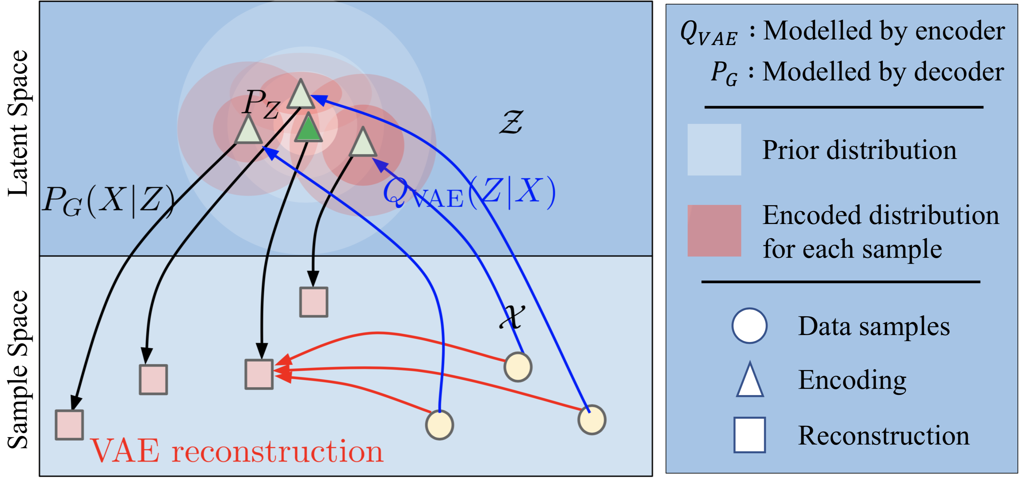
The following figure beautifully shows the problem that this formulation presents. During training, the KL loss encourages encoded distribution (red circles) for each training sample to become increasingly similar to the prior distribution (white circles). Over time, the distributions of different training samples would start overlapping and leads to the following inconsistency:
Points like the green triangle in the overlapping regions are treated as a valid encodings for all training points; but at the same time the decoder is deterministic and one-to-one!
Figure: Matching encoded distribution of each point to a prior in a VAE. Source: Wasserstein Auto-Encoders [2] with additional annotations
This inconsistency would place the goal of achieving good reconstruction fundamentally at odds with that of minimizing KL divergence. One could argue that this is usually the case with any regularization used in machine learning today. However, note that in those cases optimizing the regularization objective is not a direct goal. For instance, in case of L2 regularization used in logistic regression, we don’t really care if our model achieves a low L2 but rather that it generalizes on test data. On the other hand, for a VAE, inference directly relies on sampling from the prior distribution. Hence it is crucial that encoded distributions match the prior!
The fix: WAE
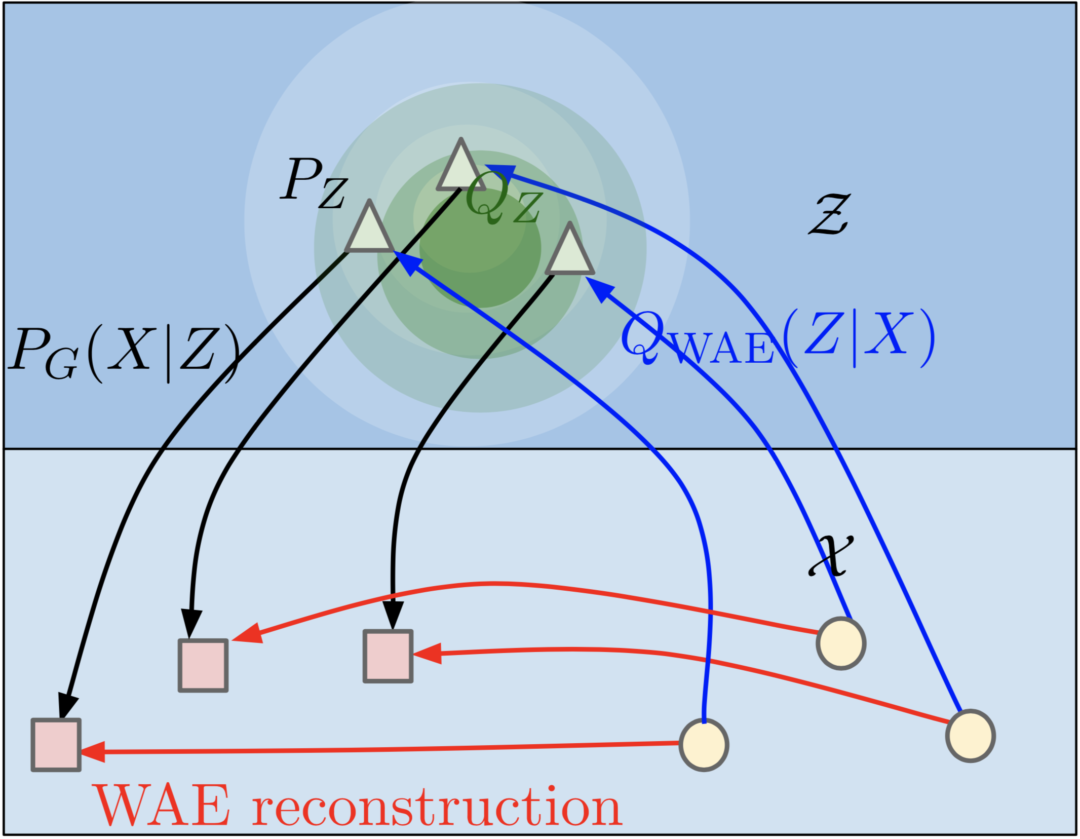
Instead of trying to match encoded distribution of each point to a prior distribution, we could match the distribution of the entire encoding space to the prior. In other words, if we took the encodings of all our training data points, distribution of those encoded points should resemble the prior distribution. WAE tries to achieve this by learning a discriminator to tell apart samples drawn from encoded and prior distributions, and training the encoder to fool the discriminator. The reconstruction loss remains intact.
Figure: Matching distribution of all training samples in the encoding space to the prior in a WAE. Source: Wasserstein Auto-Encoders [2]
SWAE
The idea behind WAE is neat, but if you have ever trained a GAN, the thought of training a discriminator should make your squirm. Discriminator training is notoriously sensitive to hyper-parameters. However, there is another way to minimize the distribution between encoded points and samples from the prior that does not involve learning a discriminator – minimizing the sliced-wasserstein distance between the two distributions. The trick is to project or slice the distribution along multiple randomly chosen directions, and minimize the wasserstein distance along each of those one-dimensional spaces (which can be done without introducing any additional parameters).
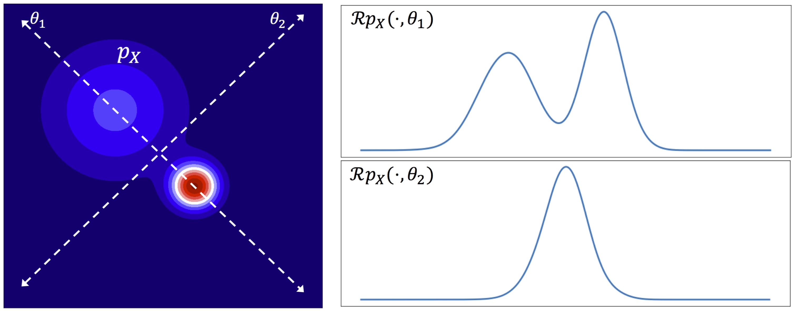
The following figure visualizes the slicing process for a 2D distribution $p_X$ along two directions $\theta_1$ and $\theta_2$. The resulting 1D distributions $\mathcal{R}_{p_X}(\cdot,\theta_i)$ for \(i \in \{1,2\}\) are shown on the right.
Figure: Slicing a distribution along randomly chosen directions. Source: Sliced-Wasserstein Auto-Encoders [3]
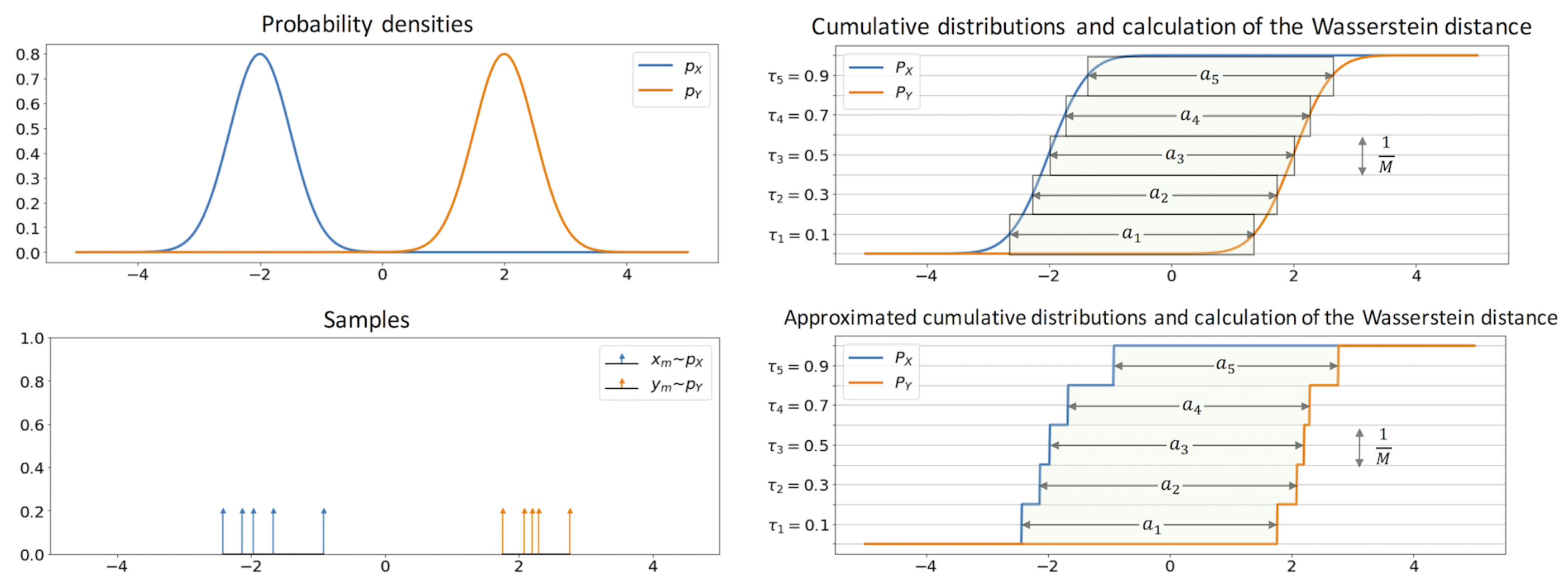
I found the following to be a very intuitive interpretation of wasserstein distance in 1D. I would recommend looking at Algorithm 1 box in 2 for a quick overview of how to compute the wasserstein distance.
Figure: The wasserstein distance is simply the area between the two CDFs shown in light green. Source: Sliced-Wasserstein Auto-Encoders [3]
Visualizing samples from trained models
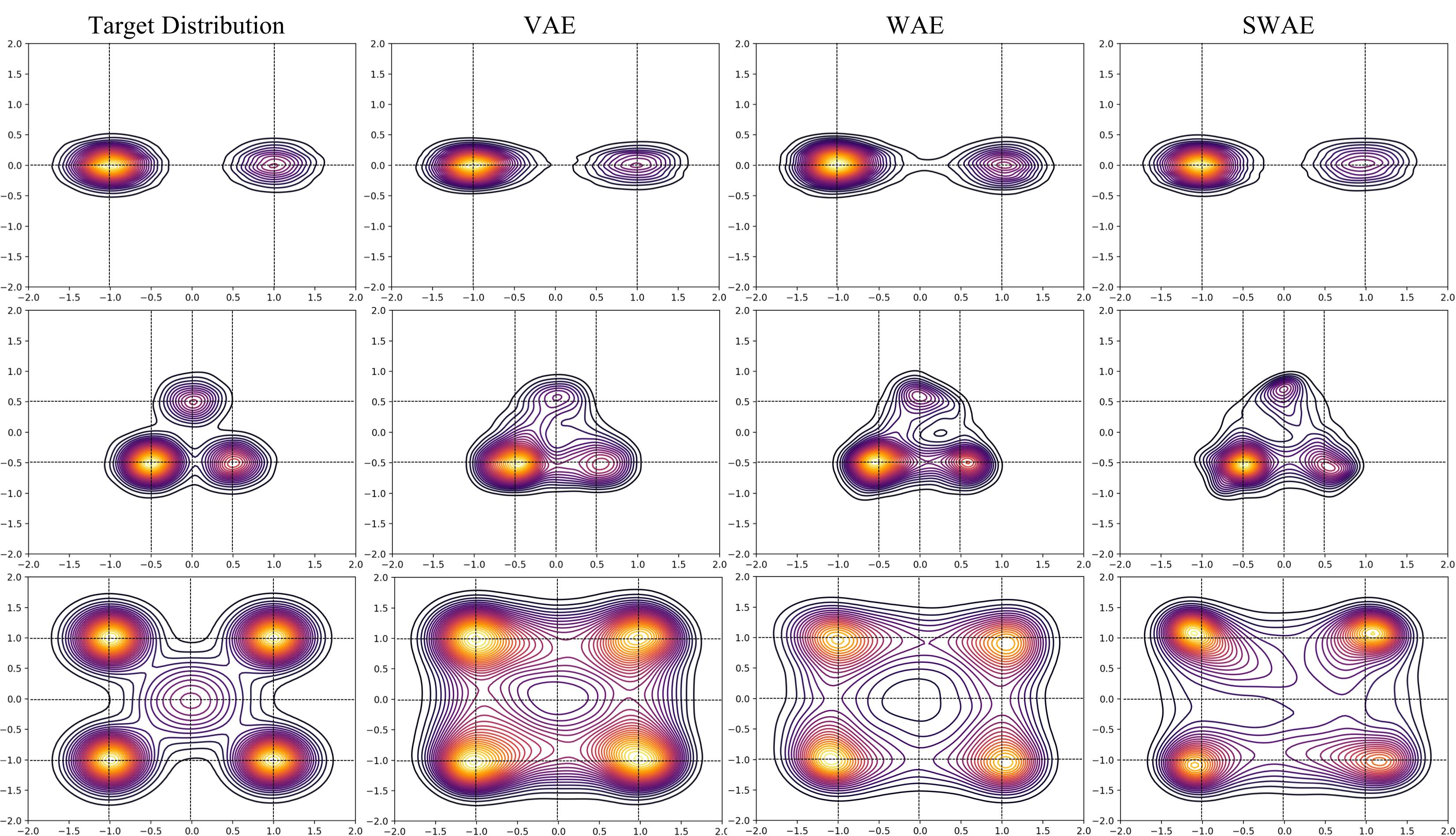
In the figure below, I have visualized samples draw from the trained models. Specifically, we are looking at contour plots of densities estimated from model samples. The density of contour lines tells us how steep the modes are, which in case of Target Distribution depends on the choice of mixing coefficients of the GMM.
From the plots above, we can make a few observations about the ability of VAE, WAE, and SWAE to learn modes. Modes are the home of the most representative samples from any distribution. Hence it is crucial to check if models learn the location of the modes as well as assign correct densities to those modes.
Mode Location: VAE has the most precise mode locations followed by WAE and then SWAE. For instance, see the mode locations (0.5,-0.5),(0.0,0.5) for the 3 component GMM, and (1,1),(1,-1) for the 5 component GMM. For the 5 component GMM, VAE and WAE missed the low density mode at (0,0). Don’t be fooled by those concentric circles around (0,0) in case of VAE and WAE! Notice how the contour lines get darker as they approach (0,0) indicating a decrease in density as opposed to the increase shown by the target distribution. SWAE doesn’t localize this mode well either but at least the density does not decrease as you approach the mode from most directions.
Mode density assignment: To gauge density assignment, we need to observe the color (yellow/lighter colors mean higher density), and also the density of contour lines which indicate how steep the peaks are. Note that VAE tends to assign significant density to the space between modes (e.g. around (0,1) in 5 component GMM) and doesn’t assign significant density to lower density modes like (0.0,0.5),(0.5,-0.5) in 3 component GMM, and (0,0) in 5 component GMM. WAE is slightly unpredictable in density assignment. For instance, WAE assigns too much density to (0.5,-0.5) in the 3 component GMM, and too little to all the high density modes in the 5 component GMM. SWAE’s densities are slightly better calibrated but it has difficulty preserving symmetries both local (around the modes), and global.
Quantitative evaluation using Anderson-Darling statistic
While informative, there is only so much you that you can tell by staring at density plots. In this section, we will present a quantitative evaluation to directly measure how similar the distribution of samples from our models are to samples from the target distributions.
Anderson-Darling statistic is used to test if two set of samples come from the same distribution or if a set of samples is drawn from a given distribution. The AD statistic between two empirical CDFs $F$ (the original distribution of data) and $F’$ (the distribution of samples from learned models) is computed as follows
where n is the number of samples used to estimate the empirical CDFs. Basically, the statistic is a weighted sum of squared differences between the two CDFs with higher weights to the tails of the original data CDF. The smaller the value of the statistic, the more confident we can be of the two sets of samples coming from the same underlying distribution.
But our data lives in 2D instead of 1D, so how do we use AD statistic? We slice! We choose a set of random directions and project both sets of samples onto these directions and compute AD statistic in the induced 1D spaces. The 1D statistics are then averaged to get a measure of dissimilarity between the 2D distributions. Note that when comparing different algorithms, we need to be careful to use the same set of random directions for projection.
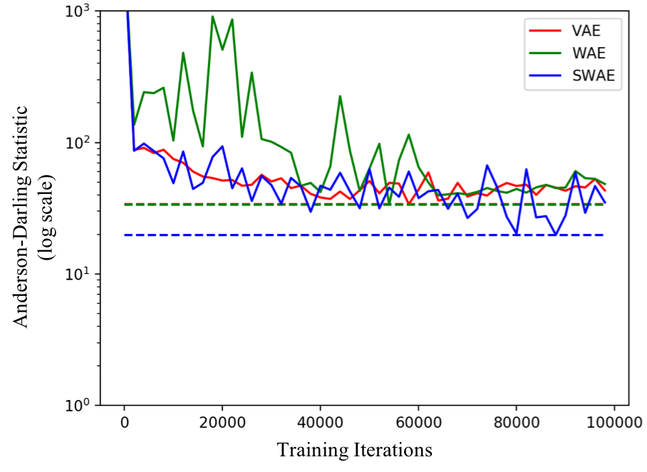
The following figure compares the AD statistic for the 3 models on the 3 distributions shown above. Smaller the statistic the better. The dotted lines show the lowest AD achieved by each model during training on the test set.
The key observations are as follows:
Best achieved performance (the dotted lines): SWAE outperforms VAE in all 3 cases. WAE outperforms VAE in 2 of the 3 cases and performs similarly in case of 5 components.
Stability of training: While SWAE and WAE perform similarly in most cases. However, in case of 3 component GMM, we see a sharp rise in AD statistic for WAE around 60000 iterations and the value plateaus to a much larger value than what was already achieved in the first 60000 iterations of training! SWAEs on the other hand are relatively more stable to train.
Encoding Space
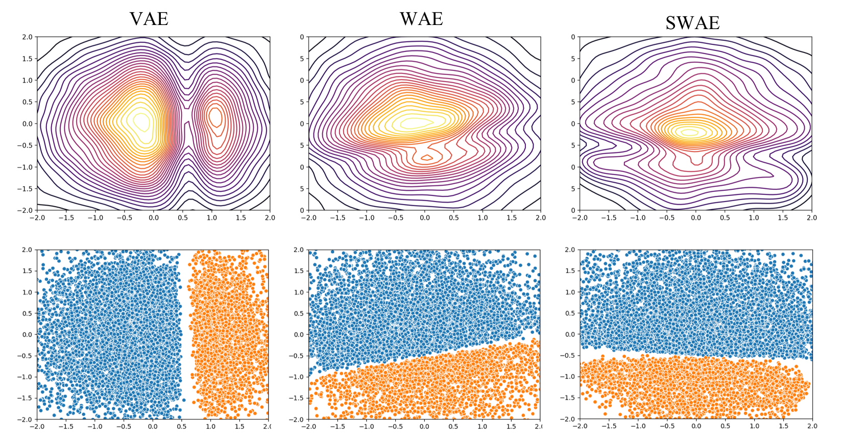
AEs and their variants are also commonly used for representation learning. VAEs, WAEs, and SWAEs, all impose constraints on this encoding or representation space. Specifically, they try to match the distribution of samples in the encoding space to that of the prior, which in our case is Standard Normal. The following plots compare the encodings from different models.
Interestingly, in all cases the components of the GMM remain well separated in the embedding space. In the 2 component case, while VAEs lead to 2 distinct modes in the encoding space, in WAE and SWAE the two modes are merged together in order to match the distribution to the Standard Normal prior. The difference is less visible in 3 and 5 component case.
The Human Factor
Any clever or sophisticated machine learning algorithm is ultimately implemented by a “human” (at least for now). So, it matters what the experience of the person implementing the algorithm is. Does the algorithm simply “work” with a “textbook” implementation at least for toy problems/data like the ones above? Or does the algorithm require “tuning” hyper-parameters? And if so, how sensitive is the algorithm to hyper-parameters - does one need to be roughly in the ballpark to get decent performance or does one need to get them just right? Is there even a signal to guide you to the right hyper-parameters?
In my experience of training these models and assuming a correct implementation, SWAEs start showing meaningful results with typical hyper-parameters! In fact, the only hyper-parameters SWAEs add to AEs is the number of slices and regularization weight. The losses are easy to interpret and help guide the hyper-parameter search. The experience with VAEs was pretty similar except that I had to adjust the weight corresponding to the KL term (the original VAEs did not have this weight but it was introduced later in $\beta$-VAEs5).
WAEs on the other hand were significantly more difficult to find hyper-parameters for. It took me a couple hours and playing with different depths of the discriminator to start seeing results that looked even remotely meaningful. The version that generated results above has a 7 layers deep discriminator which is ridiculous in comparison to my encoder and decoder which are 3 layers deep each. The discriminator is also twice as wide as the encoder and decoder. So SWAEs start appearing quite lucrative when you consider the possibility of loosing the bulky appendage that is the discriminator!
Conclusion
In this post, we discussed the problem with VAEs and looked at WAEs and SWAEs as viable recent alternatives. To compare them we visualized the distributions and encoding spaces learned by these models on samples drawn from three different GMMs. To quantify the similarity of learned distributions to the original distributions, we looked at sliced Anderson-Darling statistic.
Overall, given the conceptual and training simplicity of SWAEs, I personally found them to be a lucrative alternative to VAEs and WAEs. Completely deterministic encoder and decoders, and not requiring a discriminator during learning are two factors going in favor of SWAEs over VAEs and WAEs. SWAEs do have some problems with preserving symmetries, which the VAEs and WAEs are surprisingly good at (especially local symmetry). Hopefully, future research would fix this (one way would be by carefully choosing slicing directions instead of random).
Hope you found the discussion, visualizations and analysis informative! Please feel free to send any feedback, corrections, and comments to my email which you can find here http://tanmaygupta.info/contact/.
References
Kingma, Diederik P. and Max Welling. “Auto-Encoding Variational Bayes.” CoRR abs/1312.6114 (2014) ↩
Tolstikhin, Ilya O., Olivier Bousquet, Sylvain Gelly and Bernhard Schölkopf. “Wasserstein Auto-Encoders.” CoRR abs/1711.01558 (2018) ↩↩2
Kolouri, Soheil, Charles E. Martin and Gustavo Kunde Rohde. “Sliced-Wasserstein Autoencoder: An Embarrassingly Simple Generative Model.” CoRR abs/1804.01947 (2018) ↩
Higgins, Irina, Loïc Matthey, Arka Pal, Christopher Burgess, Xavier Glorot, Matthew Botvinick, Shakir Mohamed and Alexander Lerchner. “beta-VAE: Learning Basic Visual Concepts with a Constrained Variational Framework.” ICLR (2017). ↩
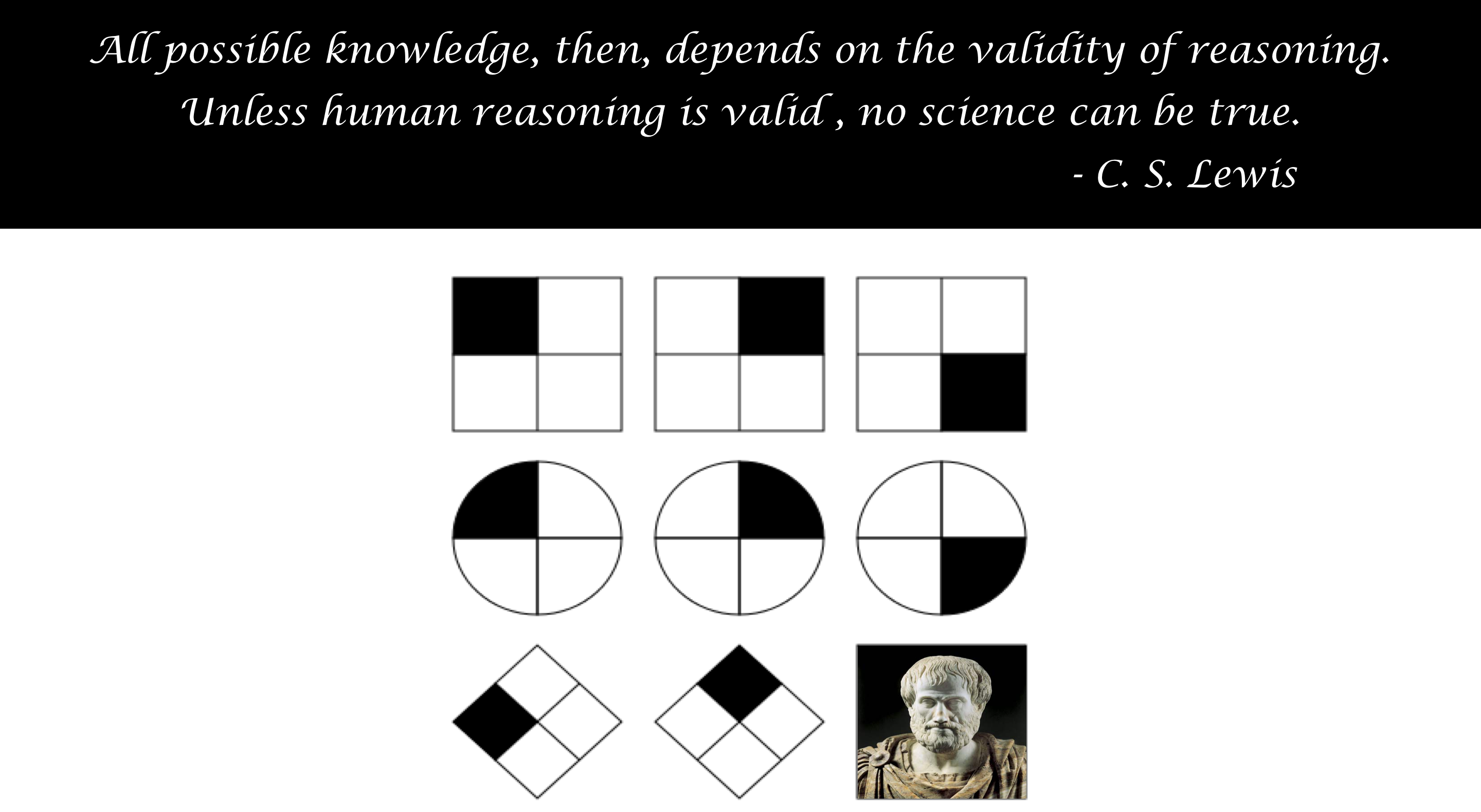
Figure: Raven's Progressive
Matrices[6] is a test used
as a measure of fluid intelligence which includes inductive and
deductive reasoning. The problem requires you to replace Aristotle
with a figure that satisfies the progression of patterns in both
vertical and horizontal directions. These are one of the many kinds of
reasoning problems that today's Visual Question Answering AI models
might struggle to solve.
By end of the first VQA challenge, most
researchers agreed that the reasoning capabilities of the first
generation VQA models were fairly limited or non-existent. Now a new
wave of models are flooding the market which attempt to address this
issue. Learning to Reason,
Inferring and Executing Programs for Visual
Reasoning, and Relation
Networks are few examples of these
next generation models. In many of these papers, authors do not
explicitly define reasoning since what they intend to convey is
often clear from context and the examples in the papers. However
reasoning is a farily complex concept with many flavors and
interesting connections to psychology, logic, and pattern
recognition. This warrants a more thorough discussion about what it
means to reason in the realm of AI and that’s what this post is all
about.
What does it mean to reason in layman’s terms?
A reason is any justification intended to convince fellow human
beings of the correctness of our actions or decisions.
In other words, if the sequence of steps or arguments you used to
reach a certain conclusion were shown to other people and they reached
the same conclusion without questioning any of the arguments, then
your reasons have held their ground. Note that what counts as a
valid reason is often context-dependent. For instance,
consider justifying calling a person crazy. When used in social
context, say during an argument with a friend, divergence from commonly
expected behaviour or established norms of morality is a valid
reason. But these arguments without a clinical diagnosis do not hold
any merit in the courthouse of clinical psychology.
When would we call an AI agent to be capable of reasoning?
Applying the layman’s definition, let us ask the question - What
would convince us of a machine’s actions or help us accept the
predictions coming from an AI system? Maybe the AI needs to be able
to list out the steps of inference which humans can manually inspect
and execute to reach the same prediction. But here’s a trick question -
Would we still call the agent capable of reasoning if inference
consists of only a single step of pattern matching or look up in a
database?
While it may seem counter-intuitive to some, using our definition of a reason
above, I would like to argue that such an agent may still be said to
reason in a particular domain of discourse if the following hold:
the approach makes correct predictions for any input in the domain
of discourse if the pattern matching is correctly executed,
the agent defines the pattern matching criterion in a human
understandable way that allows the item retrieved to be manually
verified to be a correct match given the criterion, and
given the definition of matching criterion, and a correct match a
human makes the same prediction.
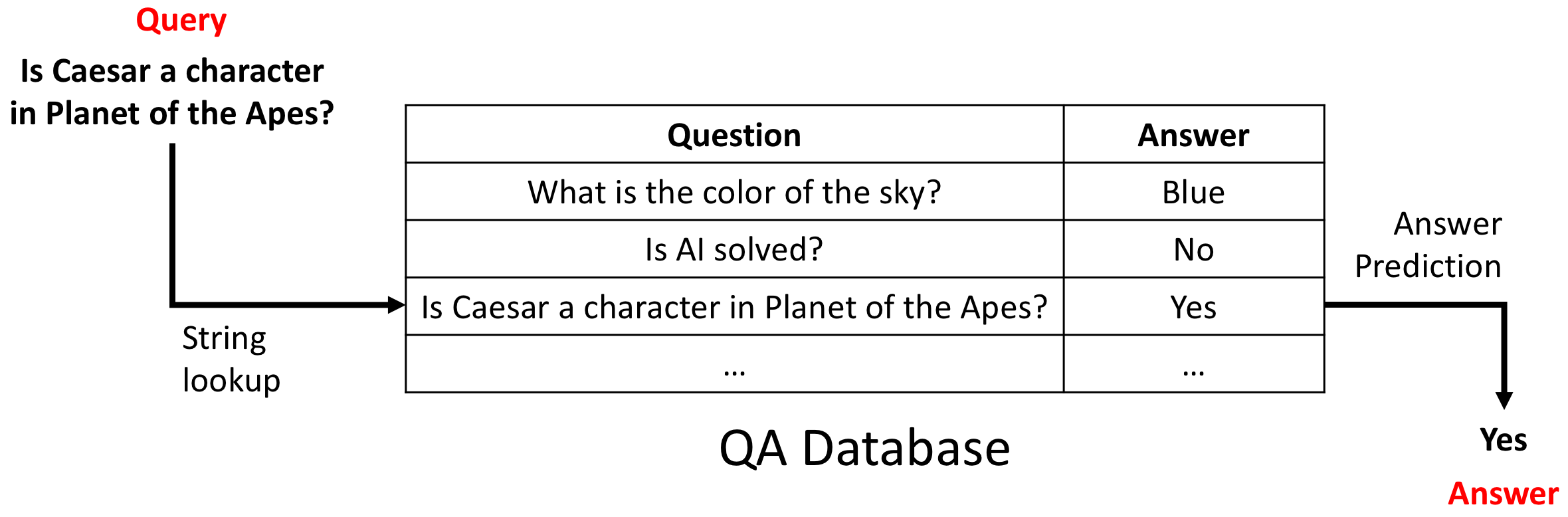
Figure: A simple reasoning QA
system.Many would not regard this as a reasoning system, but
the algorithm tells us exactly why the system made a particular prediction in a human
understandable and verifiable way. Hence the system has provided its
reasons which would be perfectly acceptable assuming the
database consists of correct QA pairs.
What this implies is that a QA system (as shown above) which only expects one of \(N\)
questions, and answers them by matching the question string to a
database of question strings paired with their correct answer string,
could be called a reasoning system. This is because the system tells
you exactly how it computed the answer in a way that can be manually
verified (does the retrieved question string match the query question
string) and executed to get the same answer. However, if we expand the
domain of discourse to include a question that is not stored in the
database, the system fails to produce an answer. Therefore, it is a
brittle system which is pretty much useless for the domains of
discourse that humans usually deal with or would like AI to deal with.
It is easy to build a system that reasons, just not one that works
for a meaningfully large domain of discourse.
Reasoning, Pattern Recognition and Composition
Taking the table lookup approach to its extreme, any reasoning
problem can be solved by a table lookup provided you could construct
a python dictionary with keys as every possible query expected with
their values being the corresponding outputs. There is a practical
problem though (you think so Sherlock!). This dictionary in most AI
applications would be gigantic if not infinitely large. Consider VQA
for example. We would need to map every possible image in the world
and every possible question that can be asked about it to an
answer. People will definitely call you crazy for trying to pull
off something like this. But this is where statistical pattern
recognition and compositional nature of the queries comes to our
rescue by helping us reduce the dictionary size.
Statistical Pattern Recognition
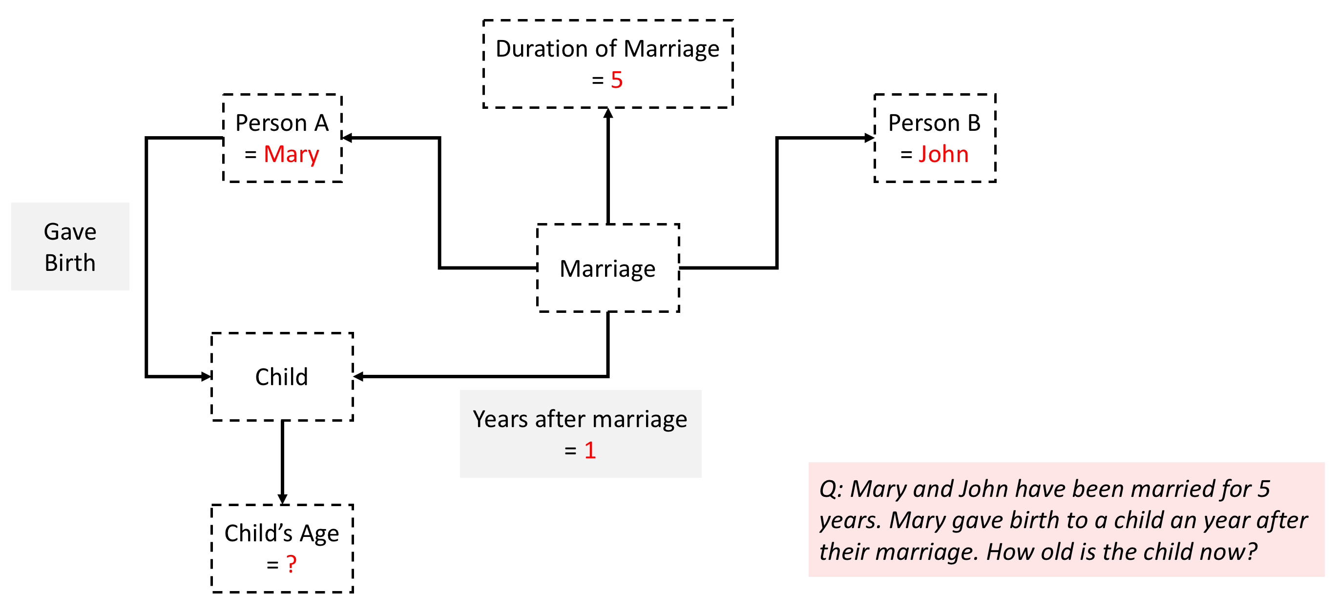
In QA a question may be posed in multiple ways using different
syntax. For example,
Mary and John have been married for 5
years. Mary gave birth to a child an year after their marriage. How
old is the child now?
and
How old is Mary and John's child now if
Mary gave birth to the child the year after they got married? They got
married 5 years ago.
are semantically the same question but the strings are quite
different. For most questions there are plenty of such semantic
duplicates. One way to reduce the size of the dictionary is to store
only one representative for each unique semantic sense and use
statistical pattern recognition (SPR) for learning a semantic
matcher instead of a simple string matcher. A naive way is encoding
sentences using an RNN trained as a language model and using nearest
neighbor lookups in the embedding space. But generally this won’t work
nearly as well as we’d hope. This is where smart ways of encoding the
sentence using parsing helps.
Composition
Composition may be though of as another aid to SPR. In the previous
example, we can replace the names Mary and John with any other
names but the meaning of the question relative to those names and its
answer doesn’t change. So the real challenge is to match the following
structure which is composed of different types of nodes and
edges. These elements combined together represent a unique semantic
sense.
Figure: Harnessing
compositional structure for reasoning.While a question may be
asked in many ways, each question with the same meaning can be mapped
to a structure comprised of primitive elements. The same primitive
elements may be found in questions with a different sense but combined
with a different set of primitives. As long as a reasoner
understands the meaning of each primitive, the meaning of any
syntactically correct novel composition can be
derived.
Further improving tractability through math and logic
So far, our lookup based approach would need to match a query to an
instantiation of this structure in terms of some or all of its
variables. For instance, in this case 5 years and 1 year are
instantiations of variables that are crucial for answering the
question. This means that in our database we need to have the question
and answer stored for every possible instantiation of variables
Duration of Marriage and Years after marriage. This observation
provides yet another opportunity for a reduction in the
dictionary size by recognizing that the answer is a formula or a
program that can be executed - Child's Age = Duration of Marriage -
Years after marriage. Useful math primitives include algebraic operators
(\(+,-,\times,\div\)), comparators (\(>,<,=\)), and logical
operators (\(\land,\lor,\neg\)). Now our inference consists of two
steps -
match question structure in the database to retrieve the
math or logical formula, and
execute the formula on the instantiation
provided by the query to get the answer.
Let’s talk implementation
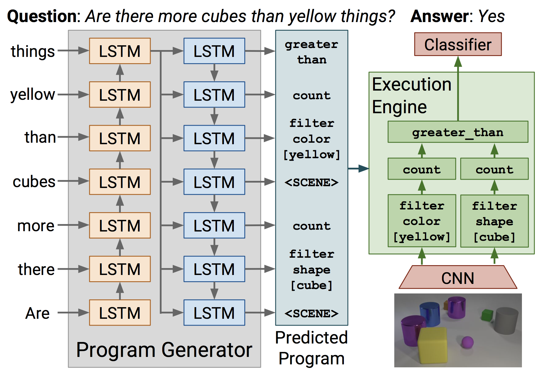
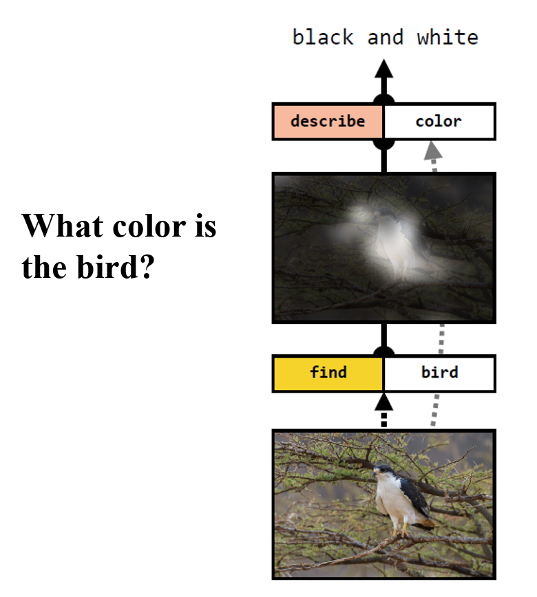
Implementation of VQA systems based on some of the above ideas can be
found in Learning to Reason and
Inferring and Executing Programs for Visual
Reasoning. Both works construct
agents which given a question about an image list a sequence of steps,
or a program if you will, that can be executed on an image to get
the answer. Each consists of passing the image or a feature map
through a neural module whose output is a feature map, an
attention map, or an answer. Each neural module is dedicated to a
certain task such as finding a particular object or attribute,
counting, comparison etc. Once assembled the modules form a network
that can be trained using backpropagation. This also leads to very
efficient data usage for learning through module reuse across
different questions.
Figure: Inferring and
Executing Programs for Visual Reasoning.[2]An RNN predicts a sequence of neural
modules which is then converted to a directed binary tree using
pre-order traversal. This DAG defines a neural architecture than is
executed on an image to predict the answer. The input and output of
each neural module are B x H x W dimensional feature maps which
conveniently allows bypassing the difficulty of ensuring compatibility
of output and input of consecutive modules.
Limitations: While these models seem quite powerful and general
enough for a large class of questions, they are not perfect. One
issues is that these models need to relearn any math or logical
operation from scratch while there is really no need to learn things
like greater_than using a neural network when most programming
languages provide > operator. Some of the operations that the
modules try to learn in a weakly supervised way, such as detection and
segmentation, have completely supervised datasets and fairly
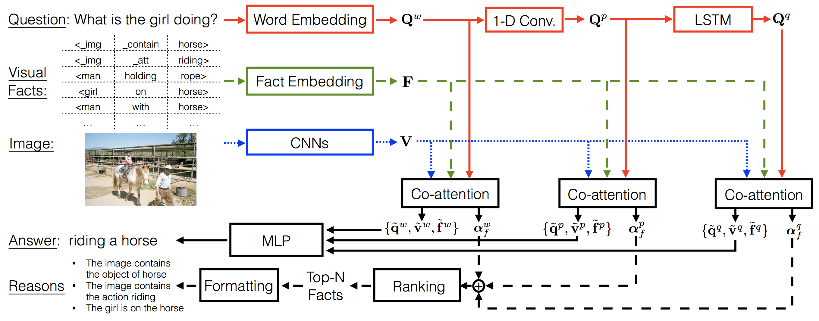
sophisticated models dedicated to these tasks alone. The VQA Machine:
Learning How to Use Existing Vision Algorithms to Answer New
Questions is a recent paper that
uses object, attribute and relationship predictions from specialized
and separately trained models as facts in VQA inference.
Figure: The VQA Machine:
Learning How to Use Existing Vision Algorithms to Answer New
Questions.[4]Visual relationship
predictions from a model trained specifically for this task are used
as facts while answering visual questions. The co-attention
framework of Lu et. al
is extended to attention over question words/phrases, image regions
and facts. A by-product of attention over facts is getting
interpretable reasons for VQA inference.
Another limitation of these models is
that they need the agent that predicts the program to be jump started
using some kind of imitation learning using ground truth programs
during training which more often than not are hard to come by. Albeit
once pretrained, the agents can be finetuned without ground truth
programs using REINFORCE. Again these are reasoning models because
humans can execute the program in our brains once we see an image and
get the answer to the question.
Dynamic vs static composition
An important thing to remember here is that a model doesn’t
necessarily have to be dynamic to be doing compositional
reasoning. Sometimes the explanation we seek in a reasoning model is
not instance specific or even explicit but rather baked into a static architecture. For
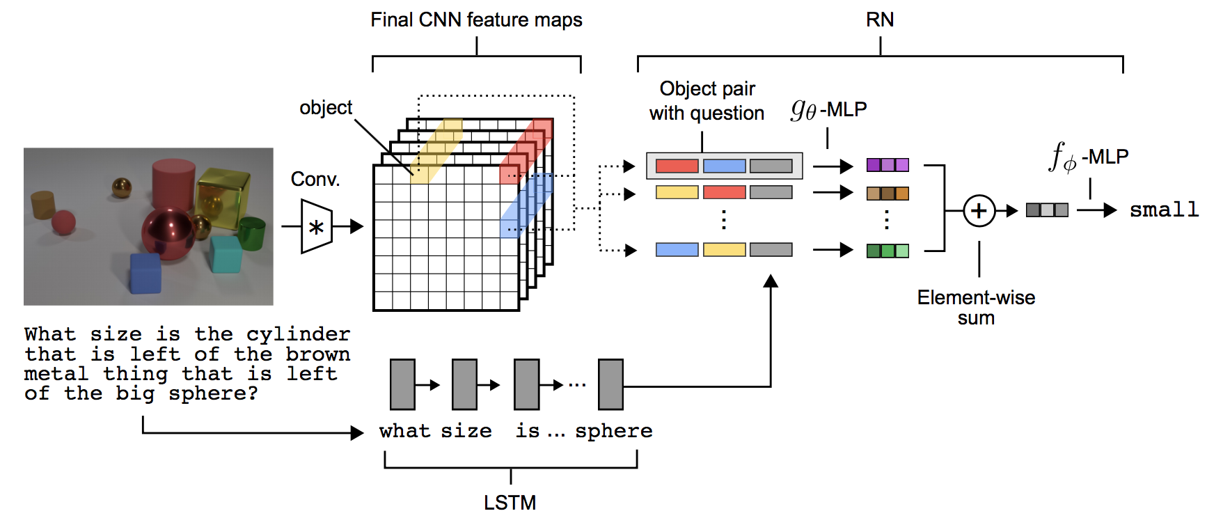
example, Relation Networks are
supposed to be doing relational reasoning but the model does not
really provide any instance specific explanation for the
predictions. However, the architecture is designed to do more than
just single-shot, black-box whole image feature extraction and
prediction. Instead the model looks at all possible pairs of regions,
encodes each region-pair and question tuple using a shared module,
pools these representations using element-wise sum, and finally makes
an answer prediction using this image representation. Here the
explanation for each prediction (and the reason why we would trust the
prediction) is that for answering questions about relations of two
objects, we would expect to get the right answer only by looking at
pairs of objects, and that is built into this particular model’s
inference but is not enforced in the first generation VQA models which
perform abysmally on relational questions.
Figure: Relation
Networks.[3]The representation of question and image used for
producing the answer is obtained by explicitly considering all
possible pairs of regions and computing
Logical operators are not the only thing that we can borrow from
formal logic to improve tractability of learning. Logic sometimes also
provides a way to encode rules and constrains learning. Since most
of machine learning deals with probabilities, we also want to encode
these rules as soft constraints. Probabilistic soft logic (PSL)
is one way to do it. To get a flavor of PSL, let us try and encode
modus ponens, which refers to the following logical rule in
propositional logic
If, $A$ is True, and $A\rightarrow B$, then, $B$ is True
Note that this can be compactly written as
$(A \land (A \rightarrow B)) \rightarrow B$
Now in PSL, \(A\) and \(B\) are not booleans but rather floating
values in the range \(\left[0,1\right]\), which could be predictions
coming from a network with sigmoid activation in the last layer. This
allows operations like \(\land\) and \(\rightarrow\) to be computed
using simple math operations such as
$A \land B \implies \text{max}\{A+B-1,0\}$
$A \lor B \implies \text{max}\{A+B,1\}$
$\neg A \implies 1-A$
$A \rightarrow B \implies \neg A \lor B \implies \text{max}\{1-A+B,1\}$
with corresponding colors denoting $(A
\land$$(A\rightarrow B)$$)$. This means that if we have probabilistic
truth values of $A$ and $B$, we can plug it into the above equation
and get a value between $[0,1]$ with $1$ indicating the rule being
exactly satisfied and $0$ indicating the rule not being satisfied at
all. Note that each branch of logic - propositional logic, predicate
logic etc. provides a bunch of these general rules of
inference. But depending on the problem, one may be able to come up
with specific logical rules. For example, an object detector might
find it useful to know that cats don’t fall from the sky (usually).
This is pretty neat, but how does one use these soft logical
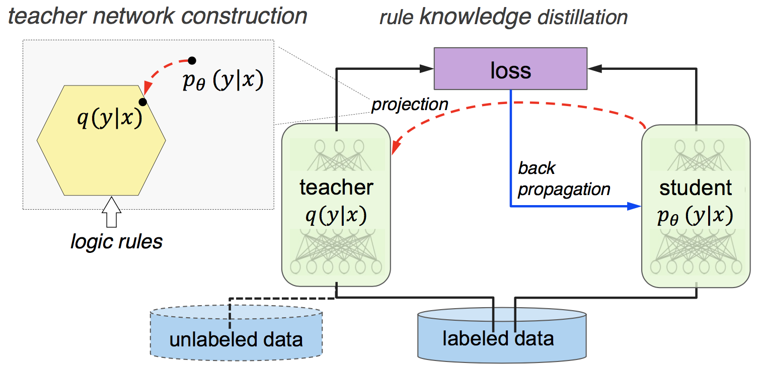
constraints in training deep networks? Harnessing Deep Neural
Networks with Logic Rules proposes
simultaneously training a student and a teacher network for
any classification task with provided PSL rules. The teacher network
projects predictions made by the student in a rule regularized
space. The student network tries to predict the correct class (cross
entropy loss) while also trying to match the predictions of the rule
compliant teacher predictions (L2 loss between teacher and student
predictions). Given, the student predictions $p_{\theta}(y|x)$ for
input $x$, and a set of rules applicable to $x$, \(\{ r_l(x,y)=1 |\;
l=1,\cdots,L \}\), the authors find a closed form solution for the
projection into the rule constrained space, which is
Figure: Harnessing Deep
Neural Networks with Logic Rules.[5]The model consists of a
teacher and a student network. The student network is
any neural network classification model. The teacher network is the
same as the student network but with an extra layer that modifies the
predictions by projecting it into a rule constrained space. The
student network tries to predict the true class while trying to match
the output of the teacher network which comply with the provided
rules. Note that the teacher network can be trained on unlabelled data
as well as long as one knows the rules that need to be applied for
each example.
What has reasoning got to do with intelligence in humans?
To answer this question, it is necessary to understand what is it that
humans call intelligence. Intelligence is commonly defined as [7]
The mental ability to learn from experiences, solve
problems, and use knowledge to adapt to new situations.
While there seems to be some concensus about its definition, the
debate about whether there is one core general intelligence or
multiple intelligences seems to be still on. The following
short video provides a comprehensive overview of 4
major theories of intelligence in psychology and the ongoing debate.
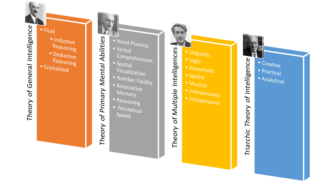
For the impatient reader who did not watch the video, below I have
summarized, the different factors associated with each theory of
intelligence. Notice that reasoning appears in some form or the other
in each theory. And just from personal experience, most people would
agree that intelligent people do effectively apply the knowledge and
skills they have already acquired to solve novel problems. But in
order to do so they need to be able to decompose any previously
solved problem into a sequence of clearly defined and easily
executable inference steps. This allows them to recognize
previously seen inference steps (or primitive operations) in novel
compositional problem structures. And then it is only a matter of
executing those inference steps correctly. Hence in some ways
reasoning allows for our finite knowledge to be applicable to
much larger set of problems than those we have already seen.
Figure: Major Theories of
Intelligence in Psychology. Reasoning is a component of all 4 major theories
of intelligence. Hence it is probably safe to assume it plays an
important role in human or artificial intelligence. The photographs
are those of the psychologists who proposed these
theories.
Conclusion
In this post our thread of thought began at a layman’s definition of
reasoning. We used the layman’s definition to understand reasoning in
context of artificial intelligence. There we argued that any reasoning
problem can be solved by lookup in a table containing all knowledge
man had, has, or will ever seek to have. We acknowledged the practical
ridiculousness of this idea and described how math, logic,
compositionality, and pattern recognition make the problem more
tractable (allowing us to answer more questions from smaller
databases). We briefly looked at existing systems that implement some
of these ideas. Finally just to mess with your mind, we dabbled in
psychology trying to figure out what does reasoning have to do with
intelligence in humans. It was a long and winding path. For some of
you it might have been a dive into a completely nonsensical rabbit
hole. For others it might serve to provide some
perspective. Irrespective, feel free to send me an email if you feel
strongly about any idea we discussed here, inaccuracies, comments, or
suggestions.
References
[1] Hu, Ronghang, et al. "Learning to reason: End-to-end module networks for visual question answering." arXiv preprint arXiv:1704.05526 (2017).
[2] Johnson, Justin, et al. "Inferring and Executing Programs for Visual Reasoning." arXiv preprint arXiv:1705.03633 (2017).
[3] Santoro, Adam, et al. "A simple neural network module for relational reasoning." arXiv preprint arXiv:1706.01427 (2017).
[4] Wang, Peng, et al. "The VQA-Machine: Learning How to Use Existing Vision Algorithms to Answer New Questions." arXiv preprint arXiv:1612.05386 (2016).
[5] Hu, Zhiting, et al. "Harnessing deep neural networks with logic rules." arXiv preprint arXiv:1603.06318 (2016).
Neural networks (NN) have seen unparalleled success in a wide range of
applications. They have ushered in a revolution of sorts in some
industries such as transportation and grocery shopping by facilitating
technologies like self-driving
cars and just-walk-out
stores. This has partly
been made possible by a deluge of mostly empirically verified tweaks
to NN architectures that have made training neural networks easier and
sample efficient. The approach used for empirical verification has
unanimously been to take a task and dataset, for instance CIFAR for
visual classification in the vision community, apply the proposed
architecture to the problem, and report the final accuracy. This final
number while validating the merit of the proposed approach, reveals
only part of the story. This post attempts to add to that story by
asking the following question - what effect do different architectural
choices have on the prediction surface of a neural network?
How is this blog different from other efforts to visually understand neural networks?
There are 2 important differences:
Complexity and Dimensionality of Datasets: Most works try to
understand what the network has learned on large, complex, high
dimensional datasets like ImageNet, CIFAR or MNIST. In contrast this
post only deals with 2D data with mathematically well defined decision
boundaries.
Visualizing the learned decision function vs visualizing
indirect measures of it: Due to the above mentioned issues of
dimensionality and size of the datasets, researchers are forced to
visualize features, activations or filters (see this
tutorial for an
overview). However, these visualizations are an indirect measure of
the functional mapping from input to output that the network
represents. This post takes the most direct route - take simple 2D
data and well defined decision boundaries, and directly visualize the
prediction surface.
Source Code
The code used for this post is available on
Github. Its written in
Python using Tensorflow and NumPy. One of the purposes of this post is
to provide the readers with an easy to use code base that is easily
extensible and allows further experimentation along this
direction. Whenever you come across a new paper on arXiv proposing a
new activation function or initialization or whatever, try it out
quickly and see results within minutes. The code can easily be run on
a laptop without GPU.
Data: A fixed number of samples are uniformly sampled in a 2D
domain, \([-2,2] \times [-2,2]\) for all experiments presented
here. Each sample \((x,y)\) is assigned a label
using \(l=sign(f(x,y))\), where \(f:\mathbb{R}^2 \rightarrow
\mathbb{R}\) is a function of you choice. In this post, all results
are computed for the following 4 functions of increasing complexity:
\(y-x\)
\(y-|x|\)
\(1-\frac{x^2}{4}-y^2\)
\(y-\sin(\pi x)\)
NN Architecture: We will use a simple feedforward architecture
with:
an input layer of size \(2\),
\(n\) hidden layers with potentially different number of units in
each layer,
an output layer of size \(2\) that produces the logits,
a softmax layer to convert logits to probability of each label \(l
\in \{1,-1\}\).
Training: The parameters are learned by minimizing a binary
cross entropy loss using SGD. Unless specified otherwise, assume
\(10000\) training samples, a mini-batch size of \(1000\), and \(100\)
epochs. All experiments use a learning rate of \(0.01\). Xavier
initialization
is used to initialize weights in all layers.
Experiments: We will explore the following territory:
Effect of activations
Effect of depth
Effect of width
Effect of dropout
Effect of batch normalization
Effect of residual connections
Each experiment will try to vary as few factors as possible while
keeping others fixed. Unless specified otherwise, the architecture
consists of 4 hidden layers with 10 units each and relu activation. No
dropout or batch normalization is used in this barebones model.
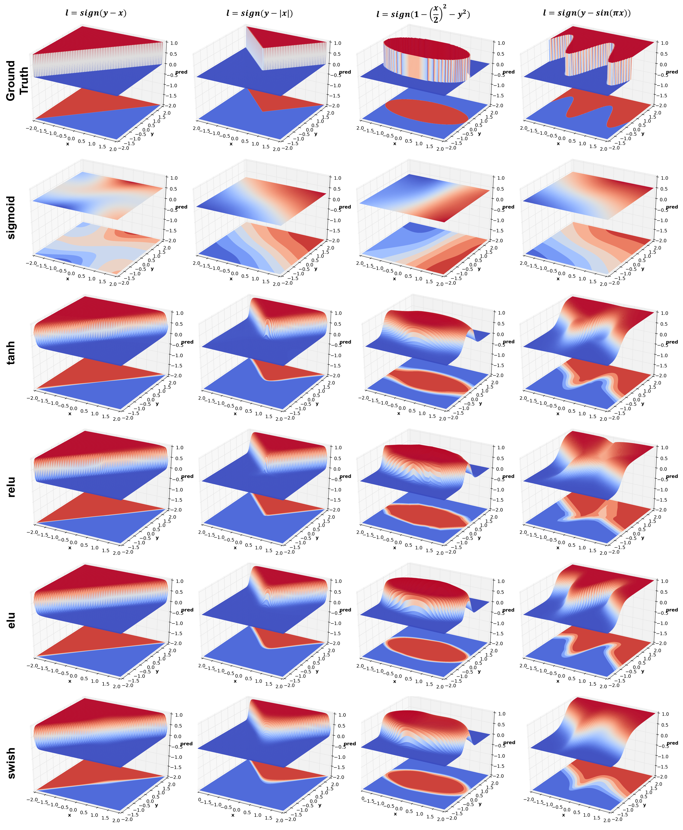
Effect of activation
This experiment compares 4 activation functions - sigmoid, tanh, relu,
elu, and the latest from Google Brain -
swish. There are a number of
interesting things to observe:
Sigmoid performs poorly. This is because of its large saturation
regions which yield very small gradients. It is possible that
results could be improved by using a higher learning rate.
Given that sigmoid fails miserably, its surprising that tanh
works so well since it has a shape similar to sigmoid but shifted
to lie between \([-1,1]\) instead of \([0,1]\). In fact tanh works
better than relu in this case. It might simply be because it
receives larger gradients than sigmoid or relu because of larger
slope (~ \(2\)) around \(0\). The elu paper also points to some
references
that provide theoretical justification for using centered
activations.
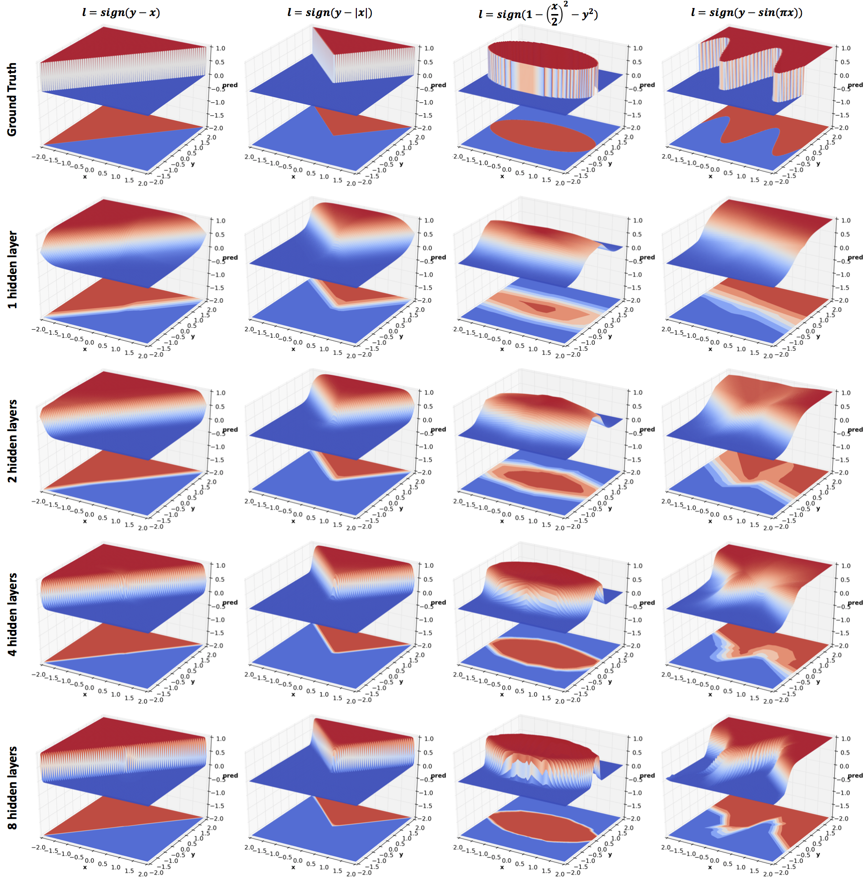
Many people don’t realize that NN with relus, no matter how
deep, produce a piecewise linear prediction surface. This can be
clearly observed in jagged contour plots of ellipse and sine
functions.
It is also interesting to compare elu and relu. While relus
turn negative input \(x\) to 0, elus instead use \(e^x-1\). See the
original elu paper for
theoretical justification of this phenomenon.
Update Oct 19 2017 - The figure above has been updated with swish, a new activation function which is a weird mix of relu and sigmoid and is defined as \(f(x) = x \cdot \text{sigmoid}(x)\). Qualitatively the results look similar to relu but smoother. Checkout the paper for more details.
Effect of depth
As mentioned in the previous section, relus produce piecewise linear
functions. From the figure above we observe that the approximation
becomes increasingly accurate with higher confidence predictions and
crisper decision boundaries as the depth increases.
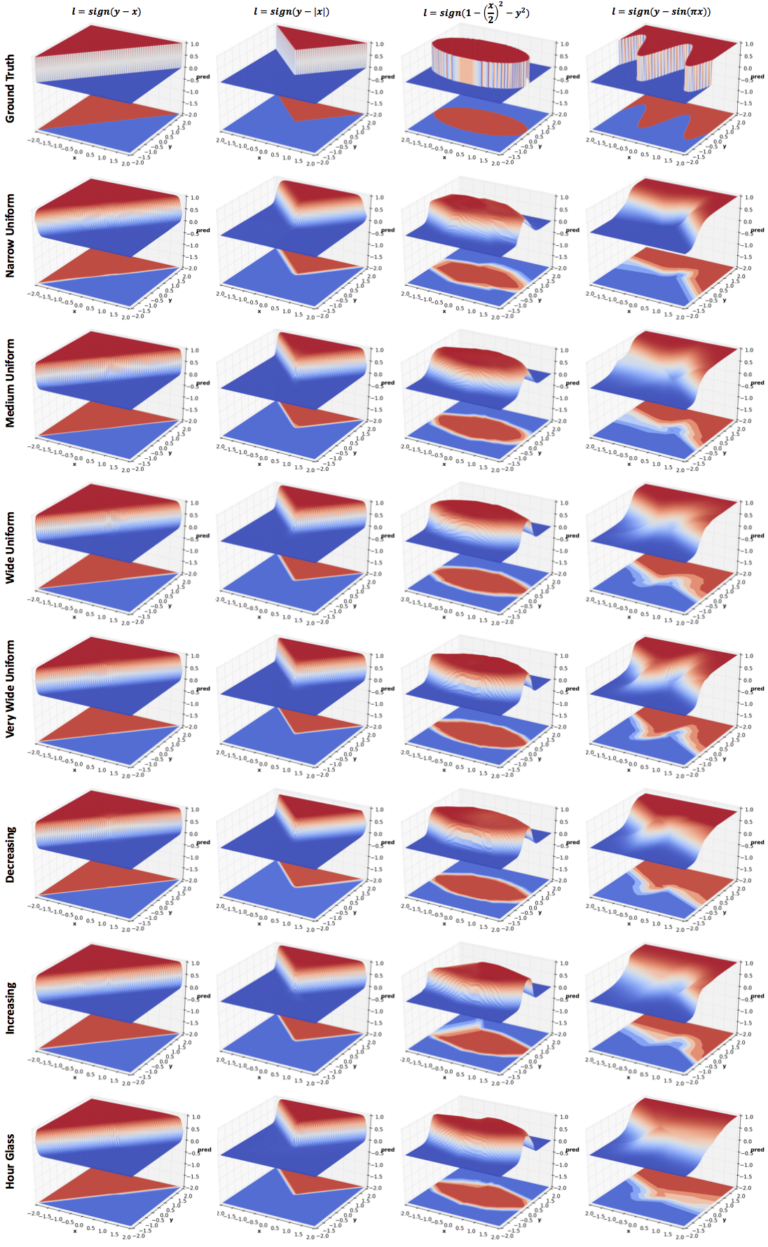
Effect of width
All networks in this experiment have 4 hidden layers but the number of
hidden units vary:
Narrow Uniform: \([5,5,5,5]\)
Medium Uniform: \([10,10,10,10]\)
Wide Uniform: \([20,20,20,20]\)
Very Wide Uniform: \([40,40,40,40]\)
Decreasing: \([40,20,10,5]\)
Increasing: \([5,10,20,40]\)
Hour Glass: \([20,10,10,20]\)
As with depth, increasing the width improves
performance. However, comparing Very Wide Uniform with 8 hidden layers
network of the previous section (same width as the Medium Uniform
network), increasing depth seems to be a significantly more efficient
use of parameters (~5k vs ~1k). This result is theoretically proved in
the paper Benefits of depth in neural
networks. One might want to reduce
the parameters in Very Wide Uniform by reducing width with depth
(layers closer to output are narrower). The effect of this can be seen
in Decreasing. The effect of reversing the order can be seen in
Increasing. I have also included results for an Hour Glass
architecture whose width first decreases and then increases. More
experiments are needed to comment on the effect of the last three
configurations.
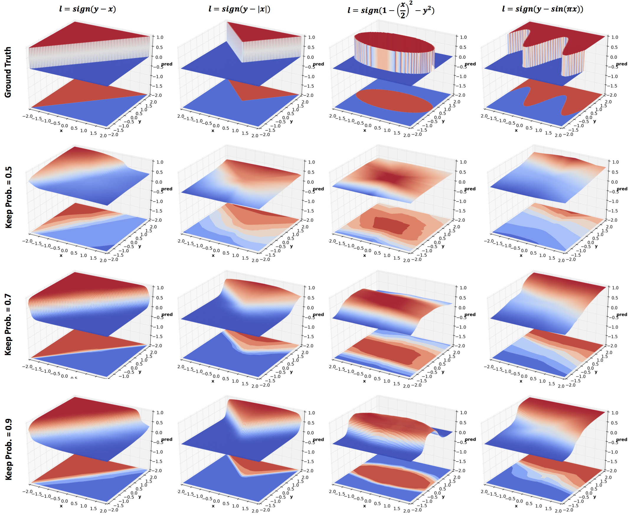
Effect of dropout
Dropout was introduced as a means to regularize neural networks
and so it does in the above results. The amount of regularization is
inversely related to the keep probability. Comparing the last row with
4 hidden layers network in the Effect of Depth section, we see quite
significant regularization effect even with a high keep
probability. But this comparison is not entirely fair since there is
no noise in the data.
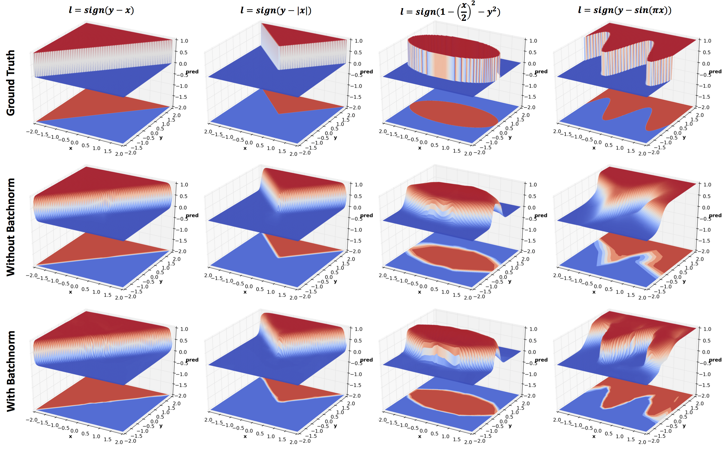
Effect of Batch Normalization
Batch normalization is reported to speed up training by a factor of 13
for ImageNet classification tasks. The above figure shows the benefit
gained by using batch normalization. You will find that this model
with batch normalization beats the 8 hidden layer network without
batch normalization in the Effect of Depth section. You can also
compare it to elu in Effect of Activations section. elu was proposed
as a cheaper alternative to Batch normalization, and indeed they
compare well.
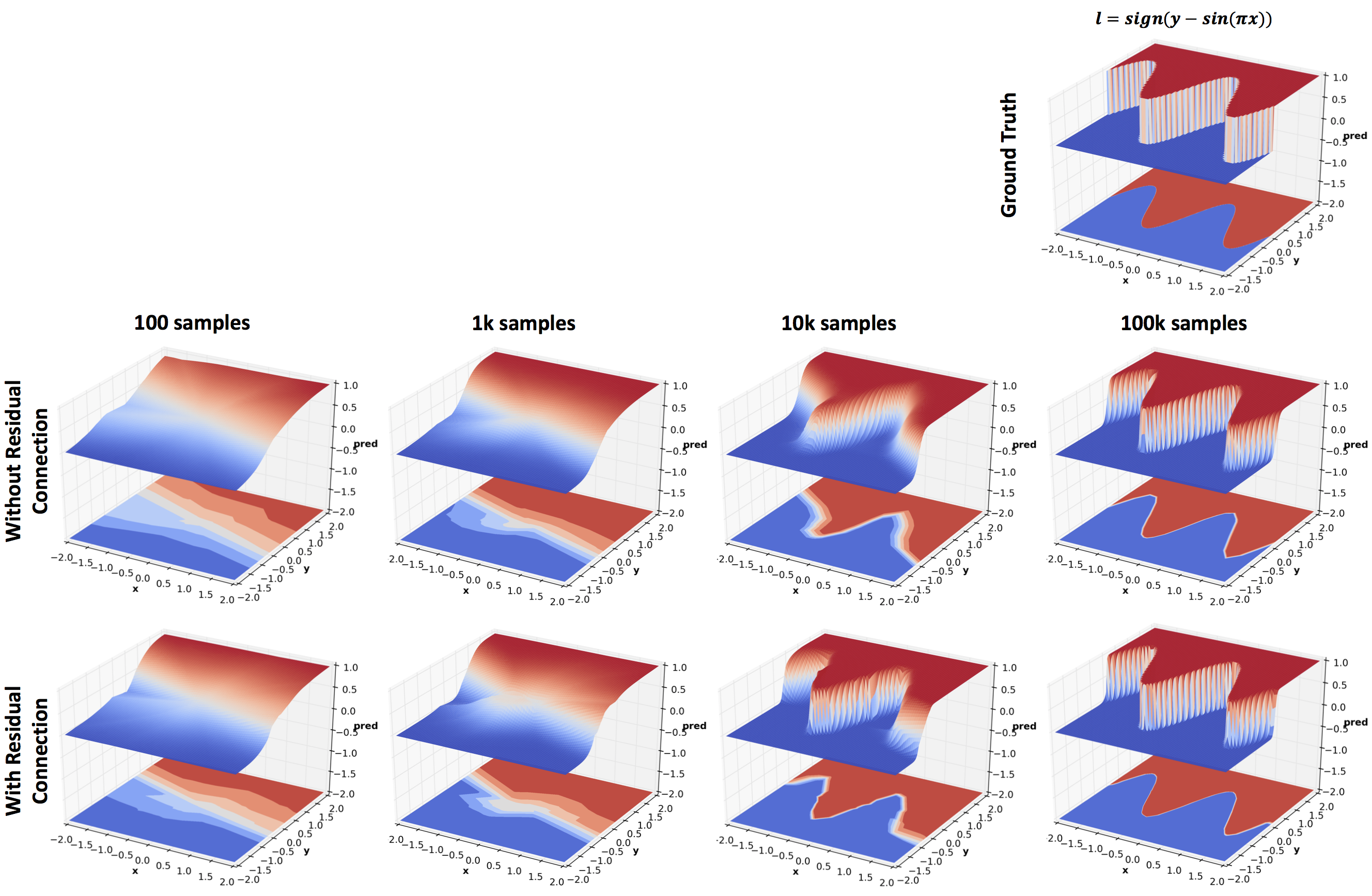
Effect of Residual Connection
The above figure compares networks with and without residual
connections trained on different number of training examples. Whenever
the input and output size of a layer matches. the residual connection
adds the input back to the output before applying the activation and
passing on the result to the next layer. Recall that the residual
block used in the original ResNet
paper used 2 convolutional layers
with relus in between. Here a residual block consists of a single
fully connected layer and no relu activation. Even then, residual
connections noticeably improve performance. The other purpose of this
experiment was to see how the prediction surface changes with the
number of training samples available. Mini-batch size of 100 was used
for this experiment since the smallest training set size used is 100.
Conclusion
Neural networks are complicated. But so are high dimensional
datasets that are used to understand them. Naturally, trying to
understand what deep networks learn on complex datasets is an
extremely challenging task. However, as shown in this post a lot of
insight can be gained quite easily by using simple 2D data, and we
have barely scratched the surface here. For instance, we did not even
touch the effects of noise, generalization, training procedures, and
more. Hopefully, readers will find the provided code useful for
exploring these issues, build intuitions about the numerous
architectural changes that are proposed on arXiv every day, and to
understand currently successful practices better.
BibTeX Citation
@misc{gupta2016nnpredsurf,
  author = {Gupta, Tanmay},
  title = {What 2D data reveals about deep nets?},
  year = {2016},
  howpublished = {https://bigredt.github.io/2017/04/21/deepvis/}
}
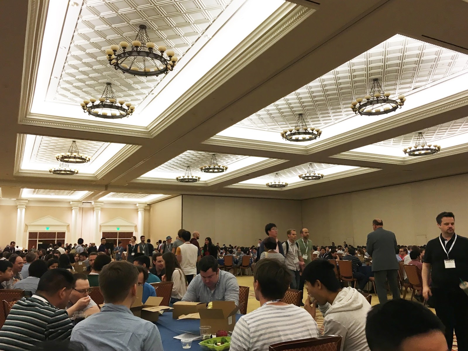
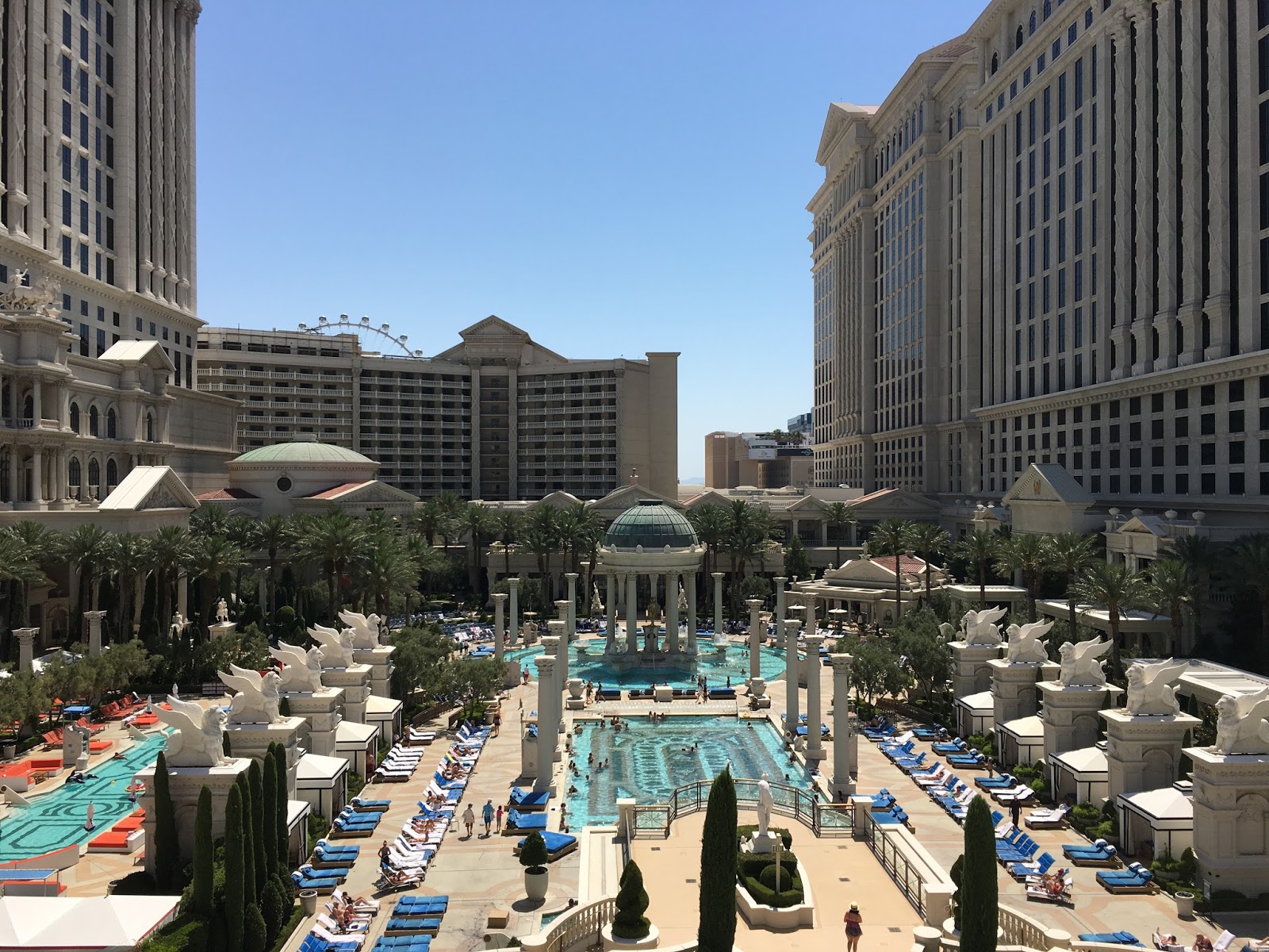
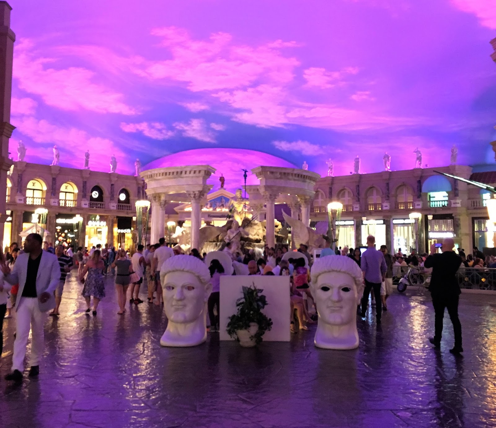
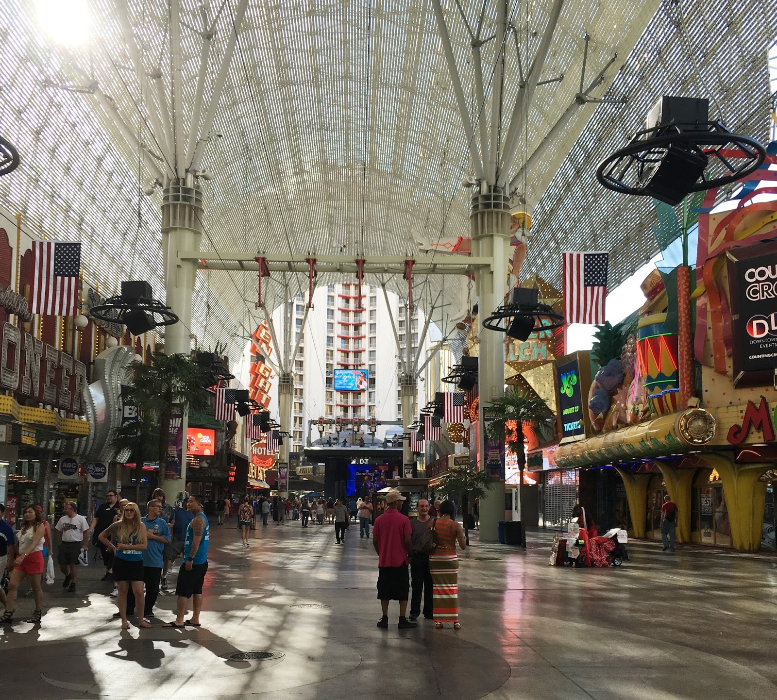
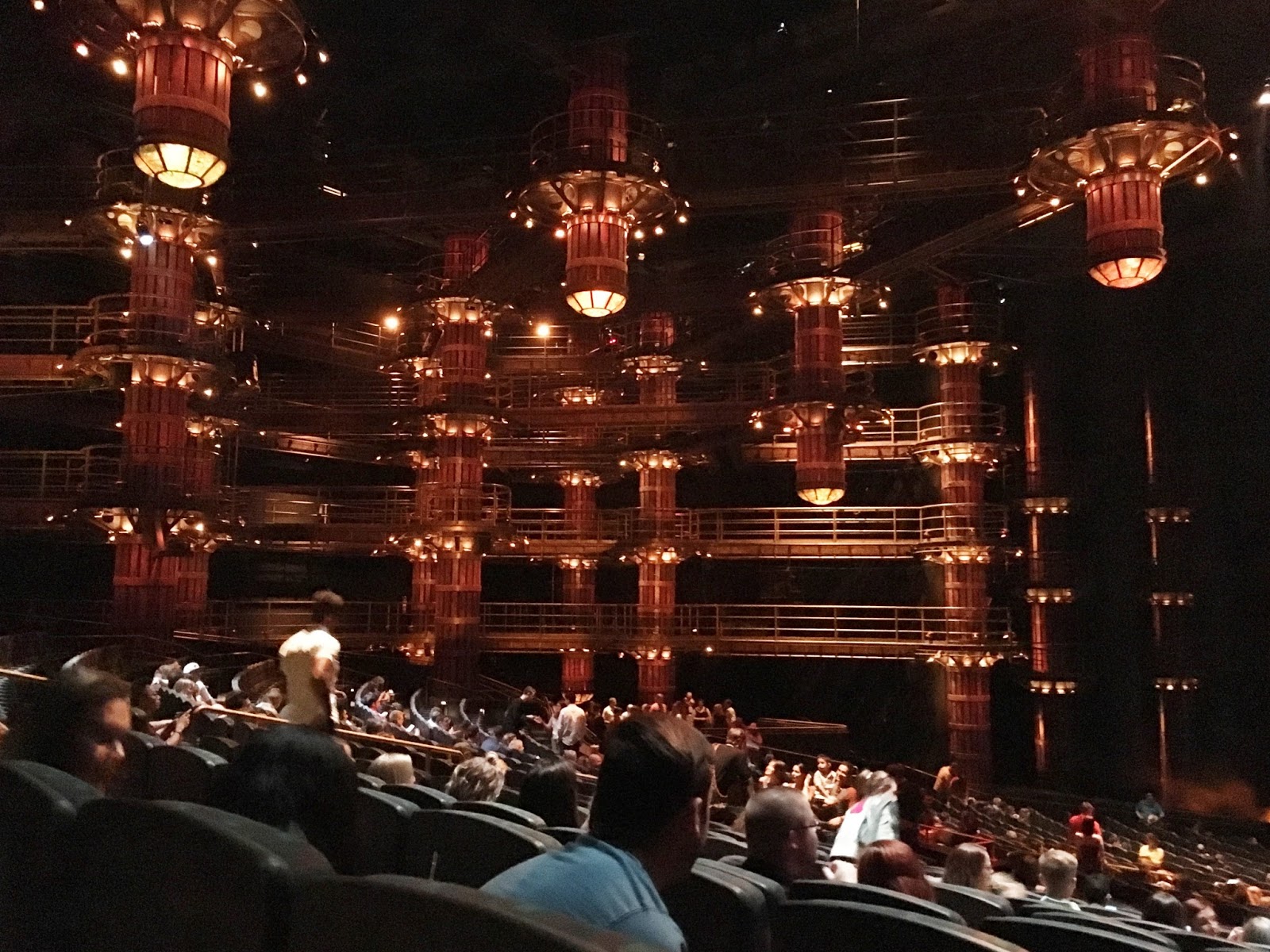
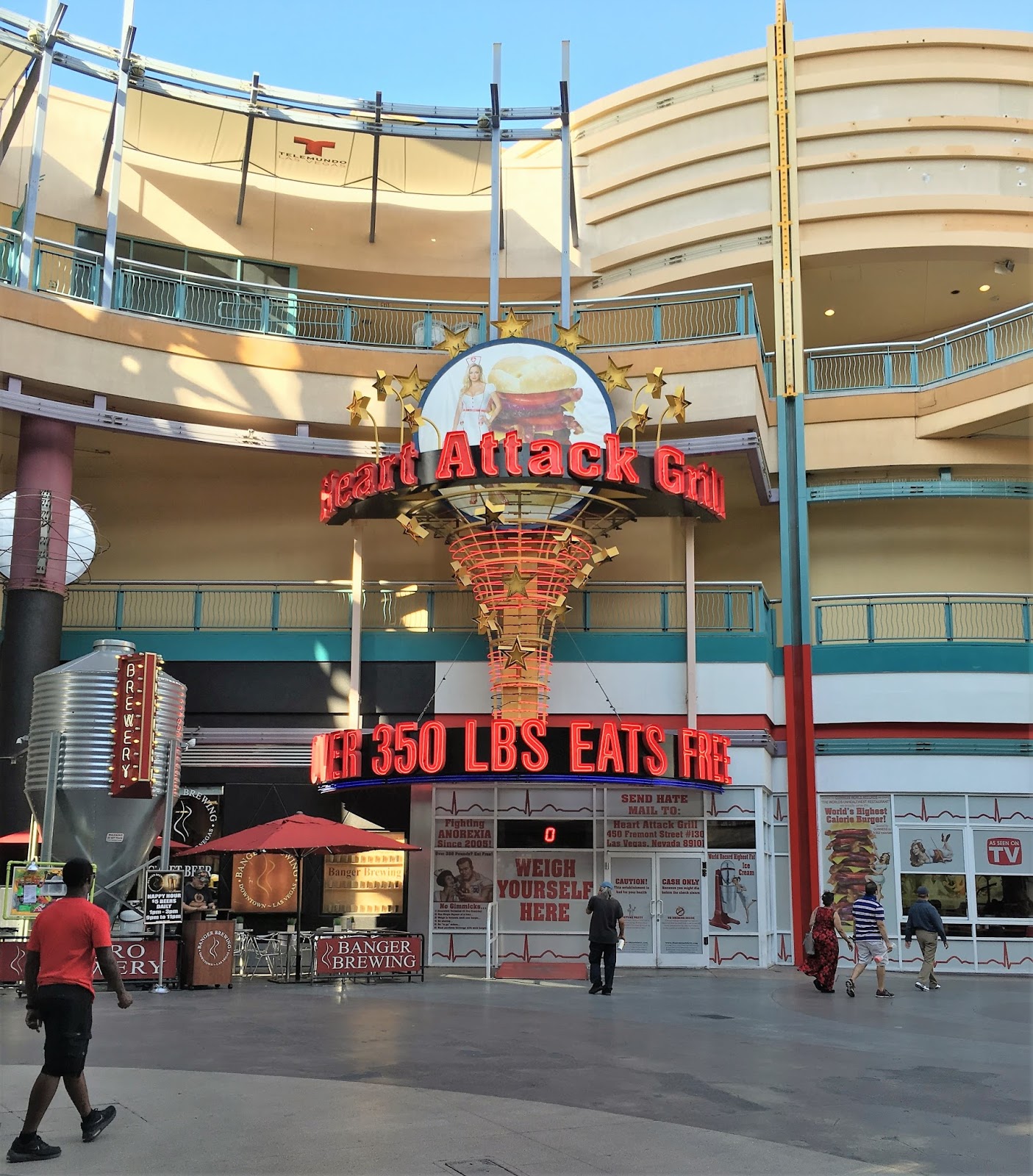
This year CVPR saw a staggering attendance of over 3600
participants. As I sat in one of those chandelier lit colossal
ballrooms of Caesar Palace (checkout some cool photos from my Vegas trip
above :smiley: ), I had only one aim in mind - to
keep an eye for honest research which is of some interest to
me. Needless to say publications featuring CNNs and RNNs were in
abundance. However it seems like the vision community as a whole has
matured a little in dealing with these obscure
learning machines and the earlier fascination with the tool itself has
been replaced by growing interest in its creative and meaningful
usage. In this post I will highlight some of the papers that seem to
be interesting based on a quick glance. This blog post is very similar
in spirit to the excellent posts by Tomasz
Malisiewicz
where he highlights a few papers from every conference he visits. I
think it is a good exercise for anyone to keep up with the breadth and
depth of a fast moving field like Computer Vision. As always many a
grad students (including me) and possibly other researchers are
waiting for Tomasz’ highlight of CVPR 2016 (which based on his recent
tweet is
tentatively named ‘How deep is CVPR 2016?’). But while we are
waiting for it let us dive in!
Vision and Language
One of the major attractions for me were the oral and spotlight
sessions on Vision and Language and the VQA workshop. There were some
good papers from Trevor Darrell’s group in UC Berkeley -
Neural Module
Network: This work
proposes composing neural networks for VQA from smaller modules
each of which performs a specific task. The architecture of the
network comes from a parse of the question which specifies the
sequence in the which operations need to be performed on the image
to answer the question. A follow up work is also available
here where instead of committing
to a single network layout, multiple layouts are proposed and a
ranking is learned using the REINFORCE rule in a policy gradient
framework.
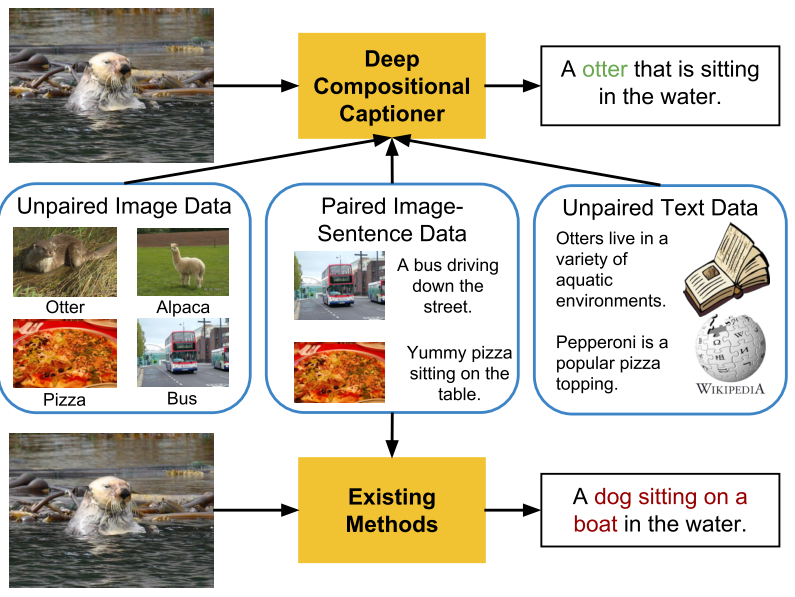
Deep Compositional Captioning: Describing Novel Object Categories
without Paired Training Data:
Most image captioning models required paired image-caption data to
train and cannot generate captions describing novel object
categories that aren’t mentioned in any of the captions in the
paired data. The main contribution of the paper is to propose a
method to transfer knowledge of novel object categories from
object classification datasets.
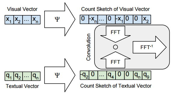
Multimodal Compact Bilinear Pooling for Visual Question Answering
and Visual Grounding:
Most deep learning approaches to tasks involving image and
language require combining the features from two modalities. The
paper proposes MCB as an alternative to simple
concatenation/addition/elementwise multiplication of the image and
language features. MCB is essentially an efficient way of
performing an outer product between two vectors and so results in
a straightforward feature space expansion.
There was also this work born out of a collaboration between Google,
UCLA, Oxford and John Hopkins that deals with referring
expressions which are expressions used to uniquely identify an
object or a region in an image -
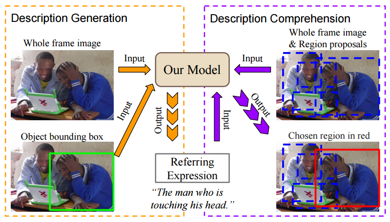
Generation and Comprehension of Unambiguous Object
Descriptions: The main
idea of the paper is to jointly model generation and
interpretation of referring expressions. A smart thing about this
is that unlike independent image caption generation which is hard
to evaluate, this joint model can be evaluated using simple pixel
distance to the object being referred to.
Shifting the attention from caption generation to use of captions as
training data for zero-shot learning, researchers from University of
Michigan and Max-Planck Institute introduced a new task and dataset in
-
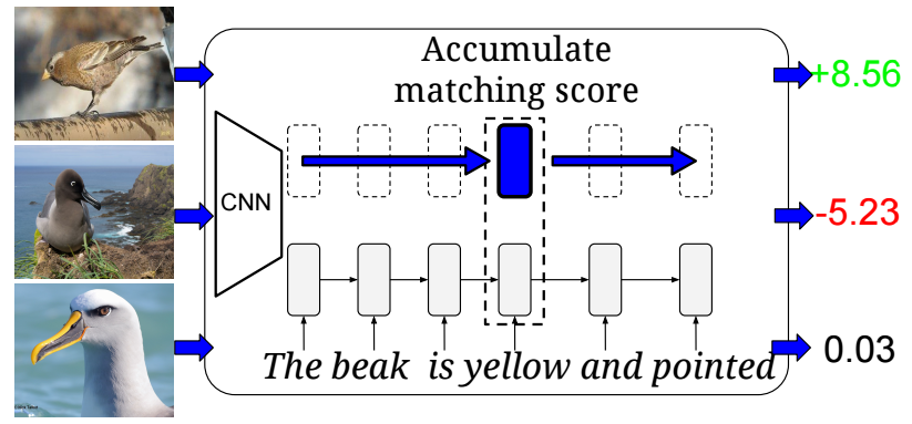
Learning Deep Representations of Fine-Grained Visual
Descriptions:
The task is to learn to classify novel categories of birds given
exemplar captions that describe them and paired image caption data
for other bird categories. The proposed model learns to score
captions and images and classifies any new bird image as belonging
to the category of the nearest neighbor caption.
During the VQA workshop Jitendra Malik brought something unexpected to
the table by pointing out that vision and language while being the
most researched pillars of AI aren’t the only ones. There is a third
pillar which has to do with embodied
cognition, the idea
that an agent’s cognitive processing is deeply dependent in a causal
way on the characteristics of the agent’s physical,
beyond-the-brain body. He argued that in order for a robot to ingrain
the intuitive concepts of physics which allow humans to interact with
the environment on a daily basis, the robot needs to be able to
interact with the world and see the effect of its actions. This theme
reflects in some of the recent research efforts lead by his student
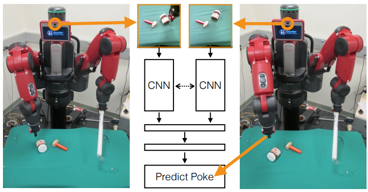
Pulkit Agrawal at UC Berkeley -
Learning to Poke by Poking: Experiential Learning of Intuitive
Physics: The main idea
here is to let a robot run amok in the world and learn to perform
specific actions in the process. In this case the robot repeatedly
pokes different objects and records the images before and after
the interaction collecting 400hrs of training data. Next a network
is trained to produce the action parameters given the initial and
final image. In this way the robot learns certain rules of physics
like the relation between force, mass, acceleration and other
factors that affect the change like friction due to a particular
surface texture. At test time, this allows the robot to predict an
action that will produce a desired effect (in this case specified
by initial and final images). Also refer to their previous work
Learning to See by Moving where
egomotion is used as supervision for feature learning.
Some other invited speakers at VQA workshop were - Ali Farhadi, Mario
Fritz, Margaret Mitchell, Alex Berg, Kevin Murphy and Yuandong
Tian. Do checkout their websites for their latest works on Vision and
Language.
Object Detection
Collaborations between FAIR, CMU and AI2 brought us some interesting
advances in object detection -
Training Region-Based Object Detectors with Online Hard Example
Mining: This work is a
reformulation of the classic hard negative mining framework that
was once popular for training object detectors with far more
negative/background samples than positive examples. The training
involved beginning with an active and possibly balanced set of
positives and negatives. A classifier trained on this active set
was applied to the complete training set to identify hard false
positives which were then added to the active set and the process
was repeated. This paper presents an online version of this
methodology which rhymes well with current object detectors like
Fast-RCNN which are trained using SGD with mini-batches.
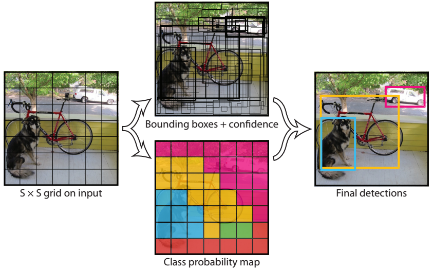
You Only Look Once: Unified, Real-Time Object
Detection: A little
pony used its
magical powers to create a really fast and simple object
detector. The key idea is to use a single forward pass through a
convolutional network and produce a fixed number of bounding box
proposals with corresponding confidence values, and class
probabilities for every cell on a grid. The pony also took great
risk but delivered a mind blowing live demo of YOLO Object
Detector during its oral session at CVPR.
Folks from ParisTech also presented their work on improving
localization of object detectors -
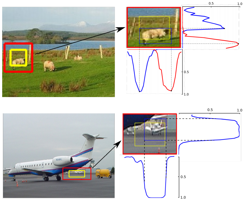
LocNet: Improving Localization Accuracy for Object
Detection: This work
proposes an approach to improve object localization. First the
initial bounding box is enlarged. Then a network is used to predict
for each row/column the probability of it belonging inside the
bounding box (or alternatively the probability of that row/column
being an edge of the final bounding box).
Recognition and Parsing in 3D
Object detection in 3D seems to be gradually catching up with its 2D counterpart -
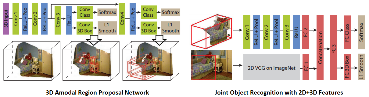
Deep Sliding Shapes for Amodal 3D Object Detection in RGB-D
Images: This paper from
Jianxiong Xiao’s group in Princeton shows how to extend the Region
Proposal Network (RPN) from Faster-RCNN to do 3D region
proposal. This region proposal is amodal meaning that the
proposed bounding box includes the entire object in 3D volume
irrespective of truncation or occlusion. For recognition they
combine deep learned 2D appearance features from image with 3D
geometric features from depth extracted using 2D/3D ConvNets
respectively.
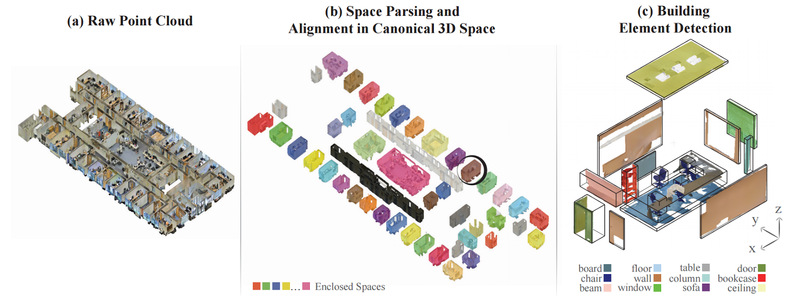
3D Semantic Parsing of Large-Scale Indoor
Spaces:
This paper due to a collaboration between Stanford, Cornell and
University of Cambridge deals with parsing of large scale 3D
scenes. For instance consider parsing an entire building into
individual rooms and hallways, and then further identifying
different components of each room such as walls, floor, ceiling,
doors, furnitures etc. The paper also suggests novel applications
that can result from this kind of parsing - generating building
statistics, analysing workspace efficiency, and manipulation of
space such as removing a wall partition between two adjacent
rooms.
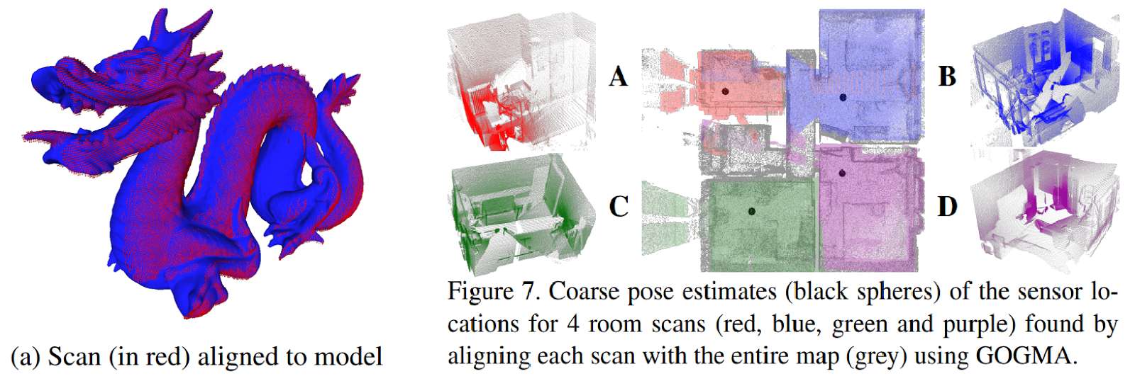
GOGMA: Globally-Optimal Gaussian Mixture
Alignment: Gaussian mixture
alignment can be used for aligning point clouds where both the
source and target point clouds are first parameterized by a GMM. The
alignment is then posed as minimizing a discrepancy measure between
the 2 GMMs. This paper presents a globally optimal solution when the
discrepancy measure used is L2 distance between the densities.
Weakly Supervised and Unsupervised Learning
With availability of good deep learning frameworks like Tensorflow,
Caffe etc, supervised learning in many cases is a no-brainer given the
data. But collecting and curating data is a huge challenge in
itself. There are even startups like
Spare5 (they also had a booth at CVPR) which
provide data annotation as a service. Nonetheless sometimes collecting
data is not even an option. Say for example the task of finding dense
correspondence between images. A dataset for this task would have a
huge impact on other tasks like optical flow computation or depth
estimation. However we are yet to see any dataset for this
purpose. The following paper has an interesting take on solving this
problem in an unsupervised fashion
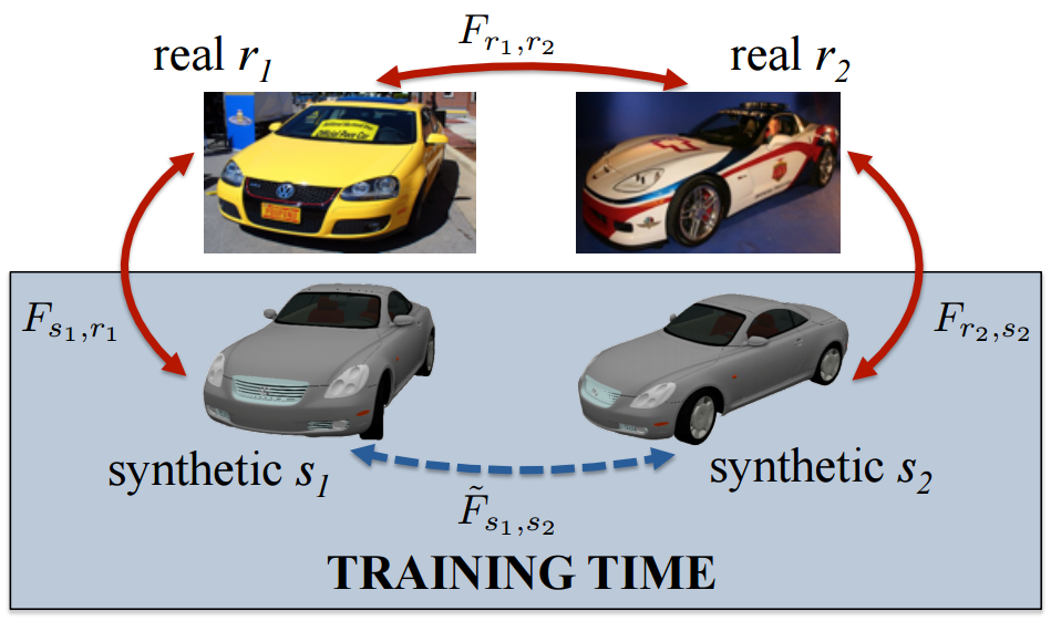
Learning Dense Correspondence via 3D-guided Cycle
Consistency: The idea in
this paper is to match both source and target real images with
images rendered from a synthetic mesh. This establishes a
consistency cycle where the correspondence between the matched
synthetic images is known from the rendering engine by
construction. This is used as a supervisory signal for training a
ConvNet that produces a flow field given source and target
images.
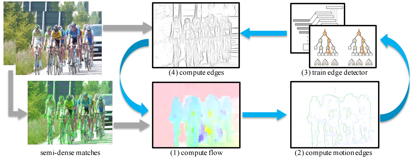
It wouldn’t be wrong to say - Piotr Dollar is to Edge Detection what Ross Girshick is to Object Detection. In this next paper Piotr and collaborators from Georgia Tech introduce an unsupervised method for edge detection -
Unsupervised Learning of
Edges: The key insight is
that motion discontinuities always correspond to edges even though
the relation does not hold in the other direction. Their algorithm
alternates between computing optical flow and using it to train
their edge detector. The output of the improved detector is then
further used to improve the optical flow and the process
continues. Over time both optical flow and edge detection benefit
from each other.
Denoising Autoencoders have been used before for unsupervised feature
learning. However depending on the noise characteristics the encoder
may not need to capture the semantics and often the clean output can
be produced from low level features. The next paper shows how to use
an encoder-decoder framework to do unsupervised feature learning in a
way that forces features to capture higher level semantics and as a
byproduct produces reasonable inpainting results -
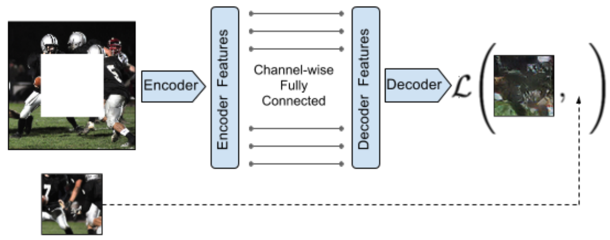
Context Encoders: Feature Learning by
Inpainting:
Given an image with a region cropped out from it, the encoder
produces a feature representation. These features are passed on to
a decoder that produces the missing region. One of their results
is that pretraining a recognition network in this fashion achieves
better performance than random initialization of weights.
The next couple papers are about weakly supervised learning where annotation is available though not in the most direct form.
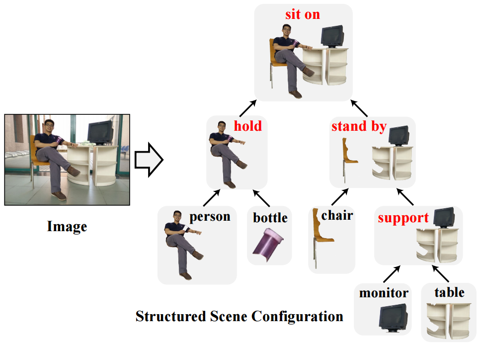
Deep Structured Scene Parsing by Learning with Image
Descriptions: The paper
proposes a method for hierarchically parsing an image using
sentence descriptions. For example given a sentence - A man
holding a red bottle sits on the chair standing by a monitor on the
table, the task is to parse the scene into something like
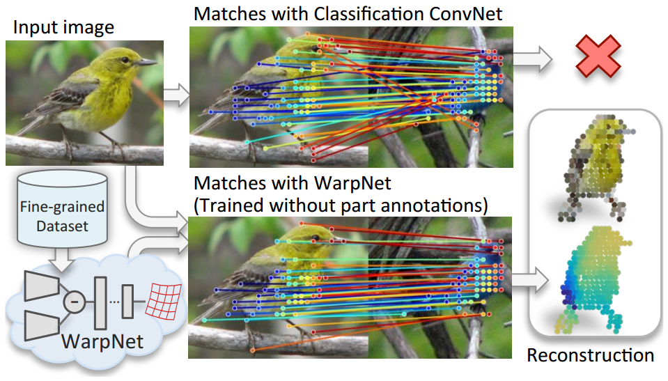
WarpNet: Weakly Supervised Matching for Single-view
Reconstruction: Consider
the problem of reconstructing a bird from a single image. One way
to do this is to use a fine grained birds dataset and use
key-point matches across instances to do non-rigid structure from
motion. However traditional key-point detectors like SIFT would
fail to give good correspondence due to appearance
variations. This paper proposes WarpNet, a network that produces a
Thin Plate Splines warping that is used as a shape prior for
achieving robust matches. Furthermore the network is trained in an
unsupervised manner without any part annotations.
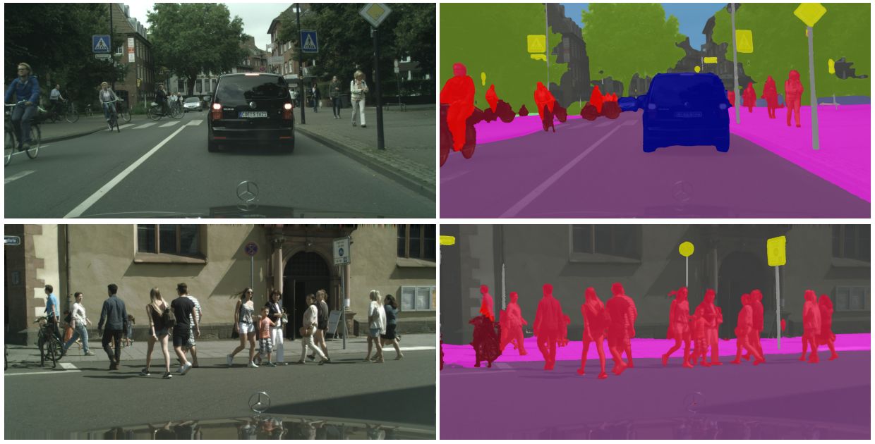
Semantic Segmentation
FCNs and Hypercolumn have been the dominant approaches for semantic
segmentation since CVPR 2015. But it is not trivial to adapt these to
instance segmentation which is the goal of the next paper-
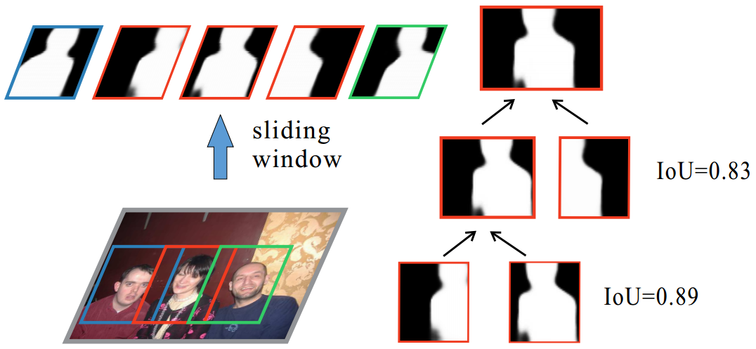
Multi-scale Patch Aggregation for Simultaneous Detection and
Segmentation:
The proposed approach is to densely sample predefined regions in
the image and for each region produce a segmentation mask
(basically foreground/background segmentation) and a
classification. The segmentation masks are then fused together to
get instance level segmentation.
In a previous
work
from Vladlen Koltun’s group, inference over fully connected CRFs was
proposed as an effective and efficient (using filtering in a high
dimensional space with permutohedral lattice) way to do semantic
segmentation. The following is an extension of that work to semantic
segmentation in videos -
Feature Space Optimization for Semantic Video
Segmentation: For semantic
segmentation in still images the fully connected CRFs could
operate in a very simple feature space - RGB color channels and
pixel coordinates. An obvious extension to video using time as an
extra feature does not work since moving objects take apart pixels
belonging to the same object in consecutive frames. The proposed
approach learns an optimal feature space over which fully
connected CRFs with gaussian edge potentials can be applied as
before.
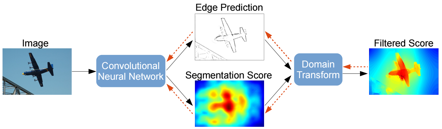
The following paper from UCLA and Google proposes an alternative to
using fully connected CRFs -
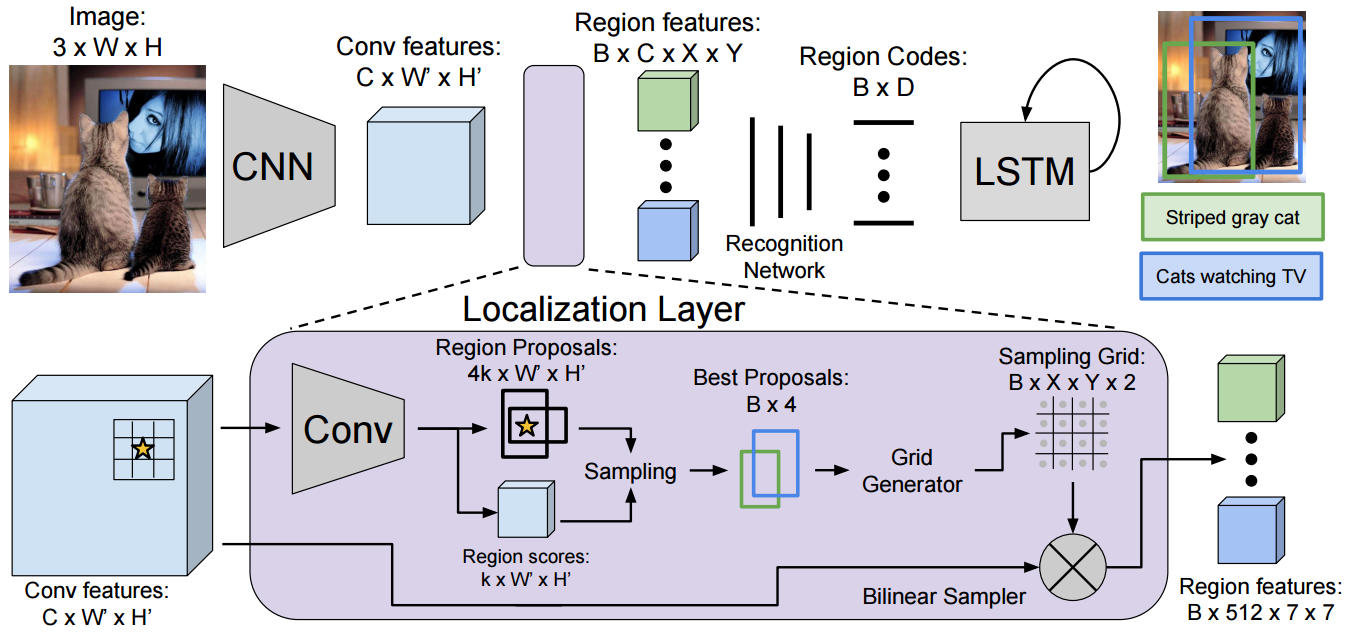
Andrej Karpathy has been a pioneer in image caption generation
technology (even though it is far from being perfect yet). In the
following paper he and Justin Johnson from Fei Fei Li’s group in
Stanford extend their captioning algorithm to generate captions
densely on an image -
DenseCap: Fully Convolutional Localization Networks for Dense
Captioning: An image is
fed into a network that produces convolutional feature maps. A
novel localization layer then takes this feature maps and produces
region proposals. Bilinear interpolation is used to get region
features from the full size feature maps which are fed into
another network with RNN at the end that generates a description
for that region.
Stereo and Monocular Vision
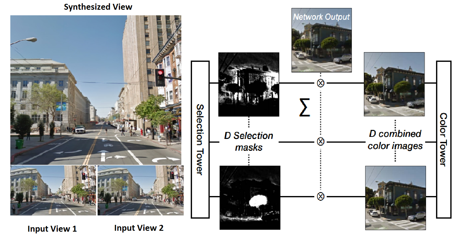
The following paper from Noah Snavely and team from Google shows us
how to generate high quality images from deep nets -
Deep Stereo: Learning to predict new views from world’s
imagery: The task is that
of novel view synthesis from a given pair of images from different
views. A plane sweep volume is feed into a network with a
carefully designed architecture that consists of a Color Tower
which learns to warp pixels and a Selection Tower which learns
to select pixels from the warped image produced by the _Color
Tower.
Current stereo depth estimation algorithms work very well for images
of static scenes with sufficient baseline. However, depth estimation
in low baseline conditions where the foreground and background move
relative to each other is still a hard problem. The next paper from
Vladlen Koltun’s group talks about dense depth estimation of scenes
with moving objects from consecutive frames captured using a monocular
camera.
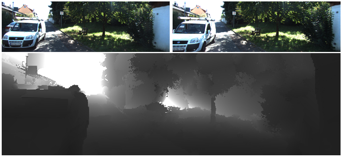
Dense Monocular Depth Estimation in Complex Dynamic
Scenes:
Due to moving objects present in the scene, the optical flow field
is first segmented. Depth is estimated using separate epipolar
geometry of each segment while enforcing the condition that each
segment is connected to the scene.