What 2D data reveals about deep nets?

Neural networks (NN) have seen unparalleled success in a wide range of applications. They have ushered in a revolution of sorts in some industries such as transportation and grocery shopping by facilitating technologies like self-driving cars and just-walk-out stores. This has partly been made possible by a deluge of mostly empirically verified tweaks to NN architectures that have made training neural networks easier and sample efficient. The approach used for empirical verification has unanimously been to take a task and dataset, for instance CIFAR for visual classification in the vision community, apply the proposed architecture to the problem, and report the final accuracy. This final number while validating the merit of the proposed approach, reveals only part of the story. This post attempts to add to that story by asking the following question - what effect do different architectural choices have on the prediction surface of a neural network?

How is this blog different from other efforts to visually understand neural networks?

There are 2 important differences:

• Complexity and Dimensionality of Datasets: Most works try to understand what the network has learned on large, complex, high dimensional datasets like ImageNet, CIFAR or MNIST. In contrast this post only deals with 2D data with mathematically well defined decision boundaries.

• Visualizing the learned decision function vs visualizing indirect measures of it: Due to the above mentioned issues of dimensionality and size of the datasets, researchers are forced to visualize features, activations or filters (see this tutorial for an overview). However, these visualizations are an indirect measure of the functional mapping from input to output that the network represents. This post takes the most direct route - take simple 2D data and well defined decision boundaries, and directly visualize the prediction surface.
  

Source Code

The code used for this post is available on Github. Its written in Python using Tensorflow and NumPy. One of the purposes of this post is to provide the readers with an easy to use code base that is easily extensible and allows further experimentation along this direction. Whenever you come across a new paper on arXiv proposing a new activation function or initialization or whatever, try it out quickly and see results within minutes. The code can easily be run on a laptop without GPU.

Data: A fixed number of samples are uniformly sampled in a 2D domain, \([-2,2] \times [-2,2]\) for all experiments presented here. Each sample \((x,y)\) is assigned a label using \(l=sign(f(x,y))\), where \(f:\mathbb{R}^2 \rightarrow \mathbb{R}\) is a function of you choice. In this post, all results are computed for the following 4 functions of increasing complexity:

1. \(y-x\)
2. \(y-|x|\)
3. \(1-\frac{x^2}{4}-y^2\)
4. \(y-\sin(\pi x)\)

NN Architecture: We will use a simple feedforward architecture with:

1. an input layer of size \(2\),
2. \(n\) hidden layers with potentially different number of units in each layer,
3. a non-linear activation function on each unit,
4. batch normalization and residual connections are used in some experiments
5. an output layer of size \(2\) that produces the logits,
6. a softmax layer to convert logits to probability of each label \(l \in \{1,-1\}\).

Training: The parameters are learned by minimizing a binary cross entropy loss using SGD. Unless specified otherwise, assume \(10000\) training samples, a mini-batch size of \(1000\), and \(100\) epochs. All experiments use a learning rate of \(0.01\). Xavier initialization is used to initialize weights in all layers.

Experiments: We will explore the following territory:

1. Effect of activations
2. Effect of depth
3. Effect of width
4. Effect of dropout
5. Effect of batch normalization
6. Effect of residual connections

Each experiment will try to vary as few factors as possible while keeping others fixed. Unless specified otherwise, the architecture consists of 4 hidden layers with 10 units each and relu activation. No dropout or batch normalization is used in this barebones model.

Effect of activation

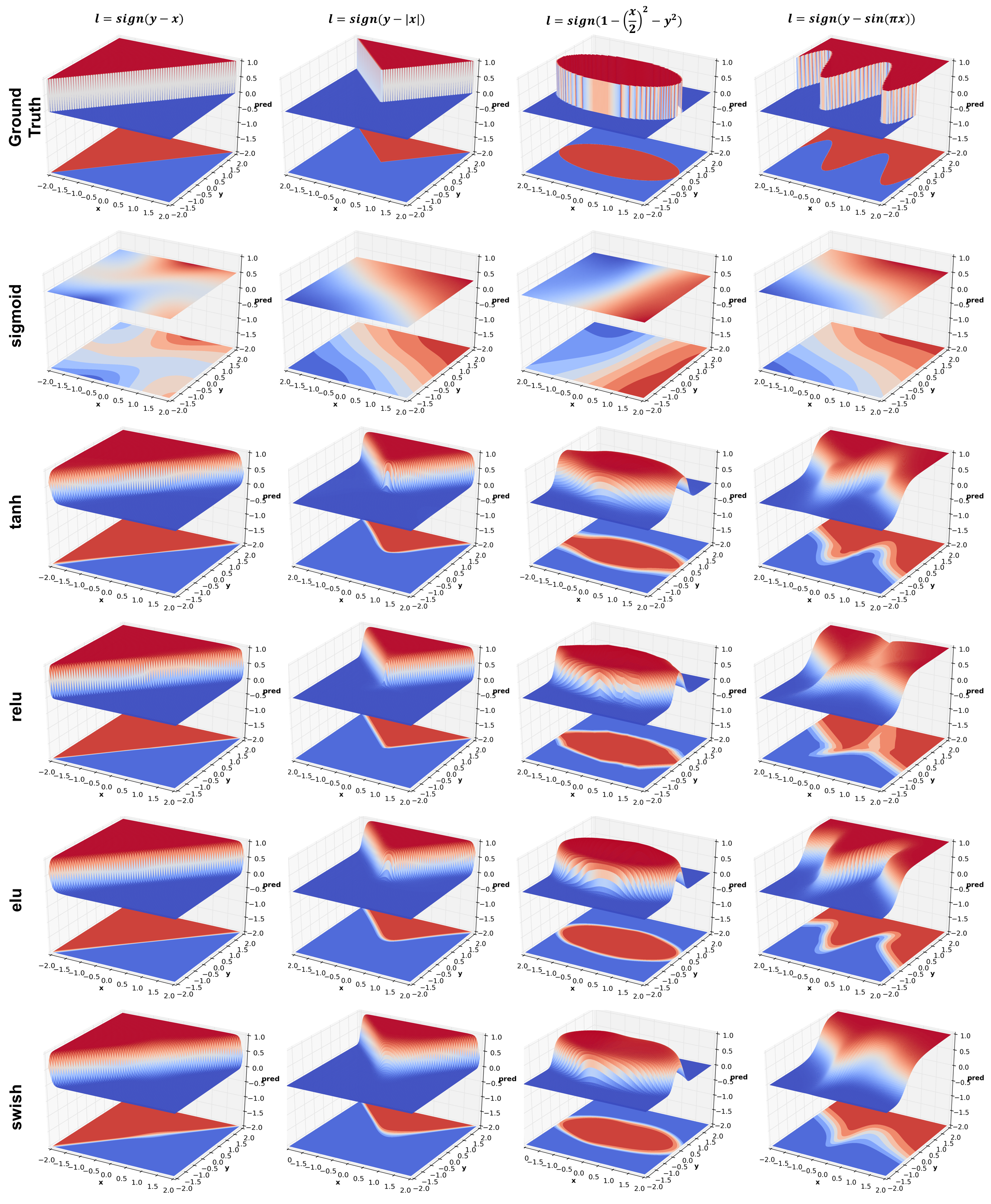
This experiment compares 4 activation functions - sigmoid, tanh, relu, elu, and the latest from Google Brain - swish. There are a number of interesting things to observe:

• Sigmoid performs poorly. This is because of its large saturation regions which yield very small gradients. It is possible that results could be improved by using a higher learning rate.
• Given that sigmoid fails miserably, its surprising that tanh works so well since it has a shape similar to sigmoid but shifted to lie between \([-1,1]\) instead of \([0,1]\). In fact tanh works better than relu in this case. It might simply be because it receives larger gradients than sigmoid or relu because of larger slope (~ \(2\)) around \(0\). The elu paper also points to some references that provide theoretical justification for using centered activations.
• Many people don’t realize that NN with relus, no matter how deep, produce a piecewise linear prediction surface. This can be clearly observed in jagged contour plots of ellipse and sine functions.
• It is also interesting to compare elu and relu. While relus turn negative input \(x\) to 0, elus instead use \(e^x-1\). See the original elu paper for theoretical justification of this phenomenon.
• Update Oct 19 2017 - The figure above has been updated with swish, a new activation function which is a weird mix of relu and sigmoid and is defined as \(f(x) = x \cdot \text{sigmoid}(x)\). Qualitatively the results look similar to relu but smoother. Checkout the paper for more details.
  

Effect of depth

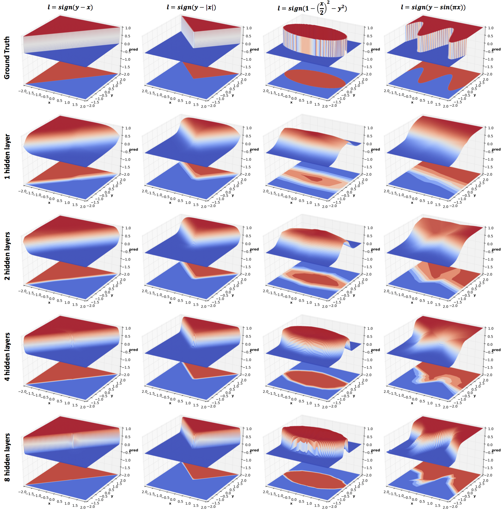
As mentioned in the previous section, relus produce piecewise linear functions. From the figure above we observe that the approximation becomes increasingly accurate with higher confidence predictions and crisper decision boundaries as the depth increases.

Effect of width

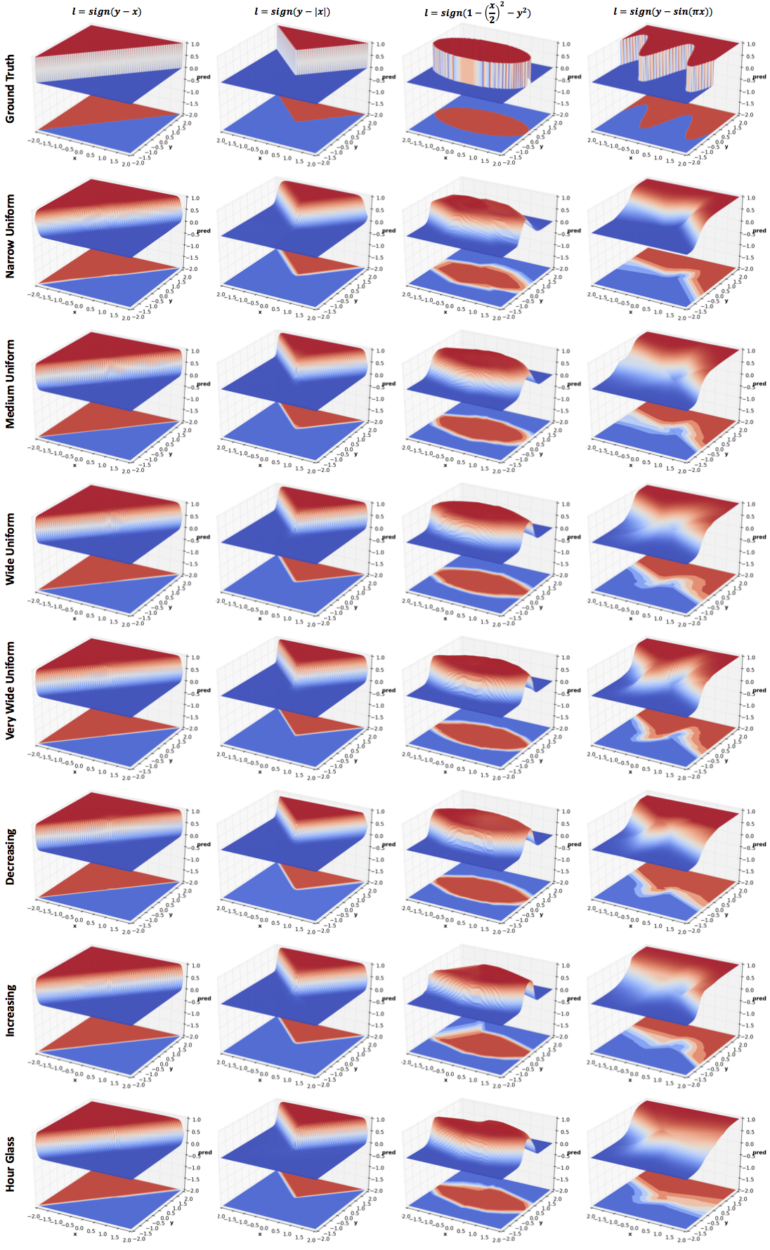
All networks in this experiment have 4 hidden layers but the number of hidden units vary:

• Narrow Uniform: \([5,5,5,5]\)
• Medium Uniform: \([10,10,10,10]\)
• Wide Uniform: \([20,20,20,20]\)
• Very Wide Uniform: \([40,40,40,40]\)
• Decreasing: \([40,20,10,5]\)
• Increasing: \([5,10,20,40]\)
• Hour Glass: \([20,10,10,20]\)

As with depth, increasing the width improves performance. However, comparing Very Wide Uniform with 8 hidden layers network of the previous section (same width as the Medium Uniform network), increasing depth seems to be a significantly more efficient use of parameters (~5k vs ~1k). This result is theoretically proved in the paper Benefits of depth in neural networks. One might want to reduce the parameters in Very Wide Uniform by reducing width with depth (layers closer to output are narrower). The effect of this can be seen in Decreasing. The effect of reversing the order can be seen in Increasing. I have also included results for an Hour Glass architecture whose width first decreases and then increases. More experiments are needed to comment on the effect of the last three configurations.

Effect of dropout

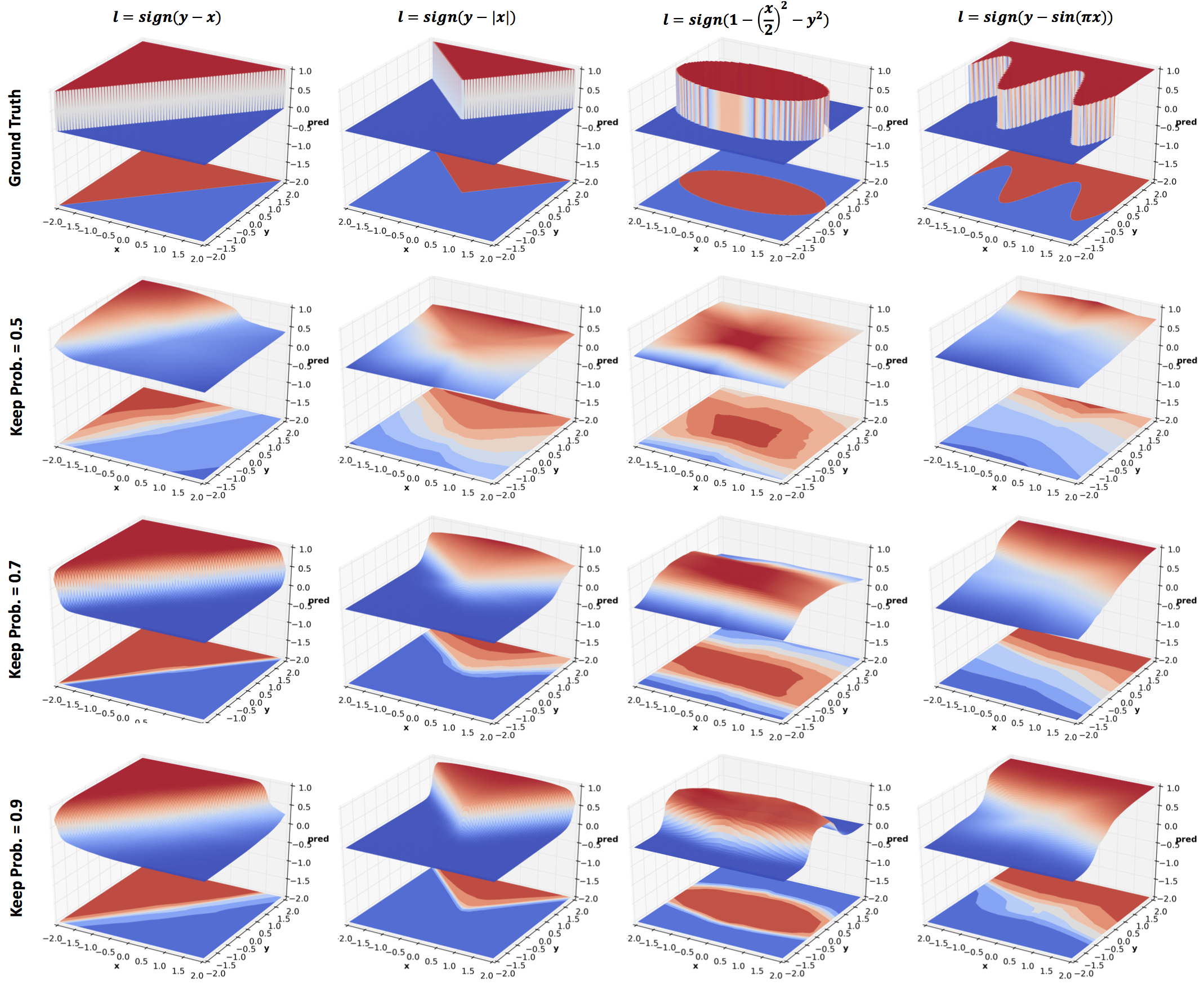
Dropout was introduced as a means to regularize neural networks and so it does in the above results. The amount of regularization is inversely related to the keep probability. Comparing the last row with 4 hidden layers network in the Effect of Depth section, we see quite significant regularization effect even with a high keep probability. But this comparison is not entirely fair since there is no noise in the data.

Effect of Batch Normalization

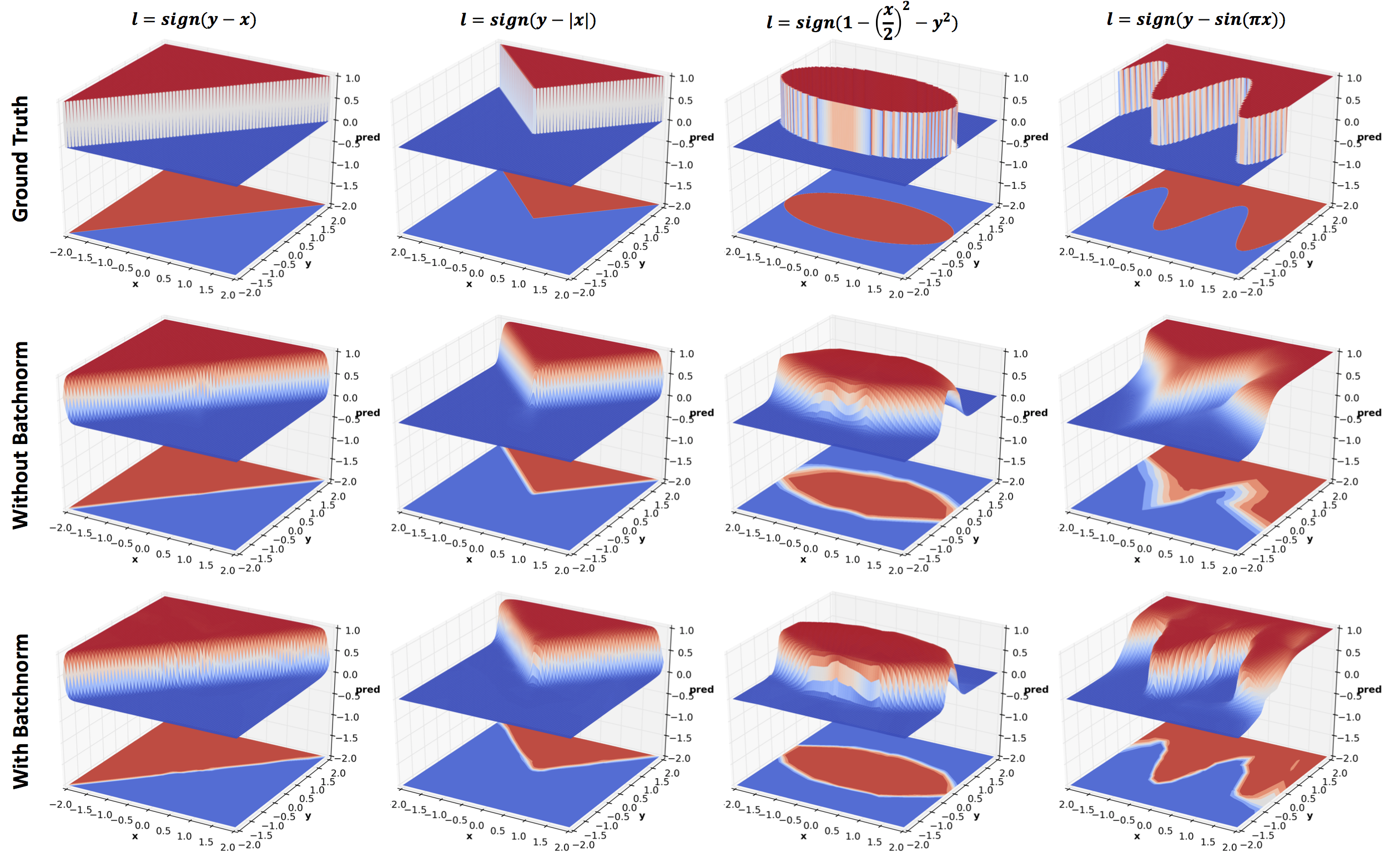
Batch normalization is reported to speed up training by a factor of 13 for ImageNet classification tasks. The above figure shows the benefit gained by using batch normalization. You will find that this model with batch normalization beats the 8 hidden layer network without batch normalization in the Effect of Depth section. You can also compare it to elu in Effect of Activations section. elu was proposed as a cheaper alternative to Batch normalization, and indeed they compare well.

Effect of Residual Connection

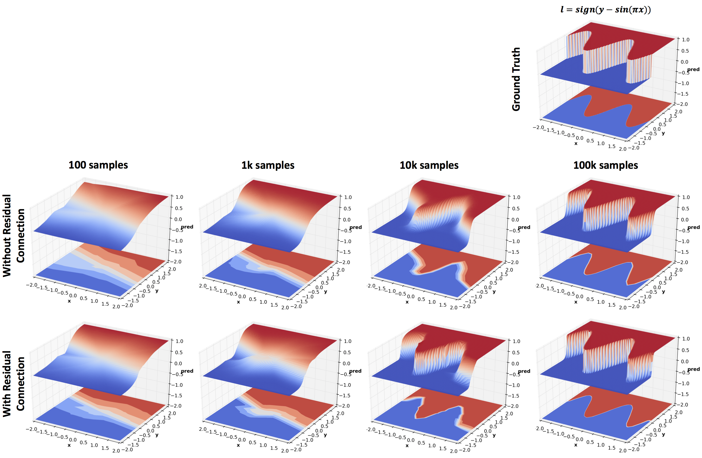
The above figure compares networks with and without residual connections trained on different number of training examples. Whenever the input and output size of a layer matches. the residual connection adds the input back to the output before applying the activation and passing on the result to the next layer. Recall that the residual block used in the original ResNet paper used 2 convolutional layers with relus in between. Here a residual block consists of a single fully connected layer and no relu activation. Even then, residual connections noticeably improve performance. The other purpose of this experiment was to see how the prediction surface changes with the number of training samples available. Mini-batch size of 100 was used for this experiment since the smallest training set size used is 100.

Conclusion

Neural networks are complicated. But so are high dimensional datasets that are used to understand them. Naturally, trying to understand what deep networks learn on complex datasets is an extremely challenging task. However, as shown in this post a lot of insight can be gained quite easily by using simple 2D data, and we have barely scratched the surface here. For instance, we did not even touch the effects of noise, generalization, training procedures, and more. Hopefully, readers will find the provided code useful for exploring these issues, build intuitions about the numerous architectural changes that are proposed on arXiv every day, and to understand currently successful practices better.

BibTeX Citation

@misc{gupta2016nnpredsurf,
  author = {Gupta, Tanmay},
  title = {What 2D data reveals about deep nets?},
  year = {2016},
  howpublished = {https://bigredt.github.io/2017/04/21/deepvis/}
}