
Generative Autoencoders Beyond VAEs: (Sliced) Wasserstein Autoencoders
Variational Autoencoders1 or VAEs have been a popular choice of neural generative models since their introduction in 2014. The goal of this post is to compare VAEs to more recent alternatives based on Autoencoders like Wasserstein2 and Sliced-Wasserstein3 Autoencoders. Specifically, we will evaluate these models on their ability to model 2 dimensional Gaussian Mixture Models (GMMs) of varying degrees of complexity and discuss some of the advantages of (S)WAEs over VAEs.
Background
Autoencoders4 or AEs constitute an important class of models in the deep learning toolkit for self-supervised learning, and more generally, representation learning. The key idea is that a useful representation of samples in a dataset may be obtained by training a model to reconstruct the input at its output while appropriately constraining (by using a bottleneck, sparsity constraints, penalizing derivatives etc.) the intermediate representation or encoding. Typically, both the encoder and the decoder are deterministic, one-to-one functions.
Variational Autoencoders or VAEs are a generalization of autoencoders that allow us to model a distribution in a way that enables efficient sampling, an inherently stochastic operation. Unlike AEs, the encoder in a VAE is a stochastic function that maps an input to a distribution in the latent space. A sample drawn from this distribution is passed through a deterministic decoder to generate an output. During training, the distribution that each training sample maps to is constrained to follow a known prior distribution that is easy to sample from, like a Normal distribution. At test time, to approximate sampling from the underlying distribution of training samples, random samples are drawn from the prior distribution and fed through the decoder (the encoder is discarded).
The problem with VAEs
VAEs involve minimizing a reconstruction loss (like an AE) along with a regularization term – a KL Divergence loss that minimizes the disparity between the prior and latent distribution predicted for each training sample. For Standard Normal distribution ($\mathcal{N}$), a commonly chosen prior, the KL loss looks like
\[E_{x\sim \mathcal{X}} \left[ D_{KL}\left(\mathcal{Q}_{VAE}(z|x) \| \mathcal{N}(z) \right) \right]\]The following figure beautifully shows the problem that this formulation presents. During training, the KL loss encourages encoded distribution (red circles) for each training sample to become increasingly similar to the prior distribution (white circles). Over time, the distributions of different training samples would start overlapping and leads to the following inconsistency:
Points like the green triangle in the overlapping regions are treated as a valid encodings for all training points; but at the same time the decoder is deterministic and one-to-one!
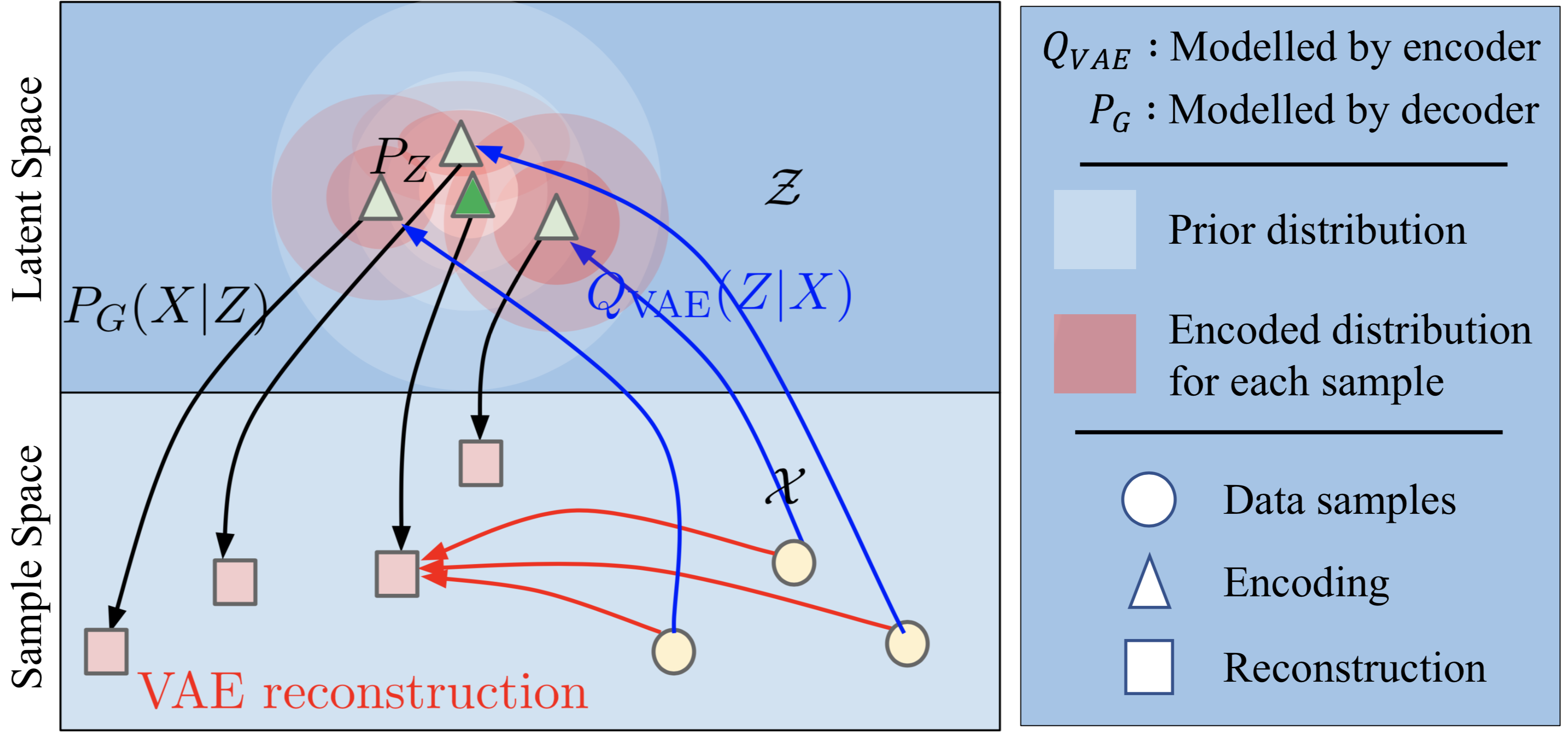
Source: Wasserstein Auto-Encoders [2] with additional annotations
This inconsistency would place the goal of achieving good reconstruction fundamentally at odds with that of minimizing KL divergence. One could argue that this is usually the case with any regularization used in machine learning today. However, note that in those cases optimizing the regularization objective is not a direct goal. For instance, in case of L2 regularization used in logistic regression, we don’t really care if our model achieves a low L2 but rather that it generalizes on test data. On the other hand, for a VAE, inference directly relies on sampling from the prior distribution. Hence it is crucial that encoded distributions match the prior!
The fix: WAE
Instead of trying to match encoded distribution of each point to a prior distribution, we could match the distribution of the entire encoding space to the prior. In other words, if we took the encodings of all our training data points, distribution of those encoded points should resemble the prior distribution. WAE tries to achieve this by learning a discriminator to tell apart samples drawn from encoded and prior distributions, and training the encoder to fool the discriminator. The reconstruction loss remains intact.
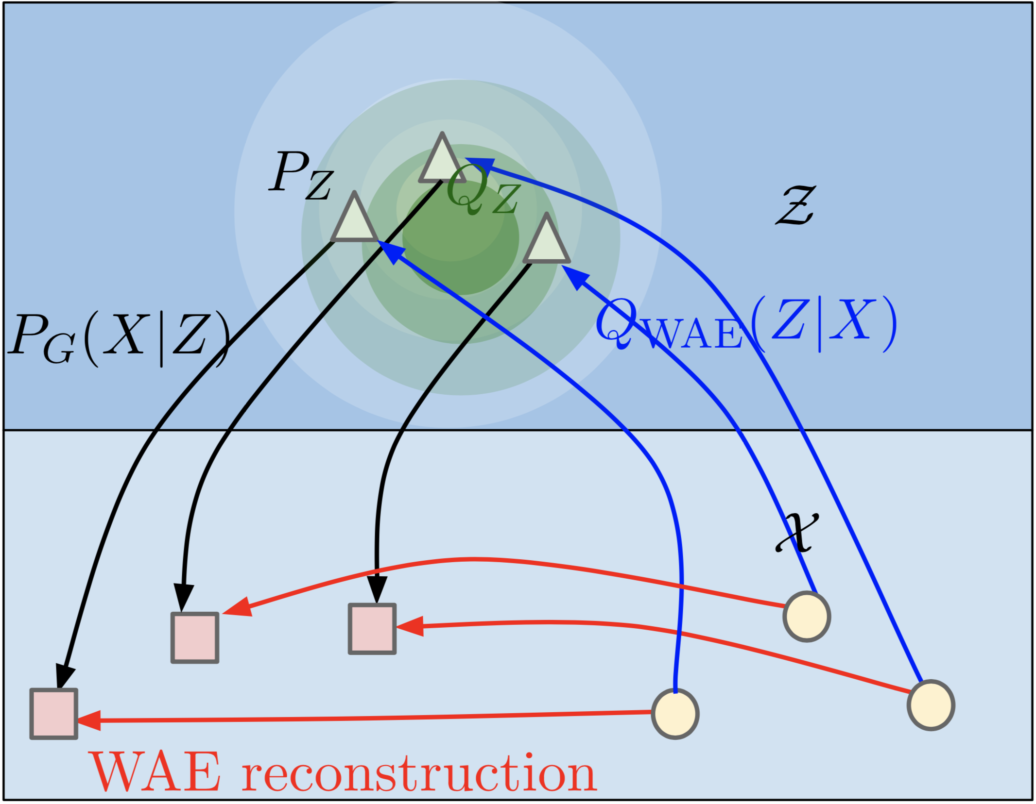
Source: Wasserstein Auto-Encoders [2]
SWAE
The idea behind WAE is neat, but if you have ever trained a GAN, the thought of training a discriminator should make your squirm. Discriminator training is notoriously sensitive to hyper-parameters. However, there is another way to minimize the distribution between encoded points and samples from the prior that does not involve learning a discriminator – minimizing the sliced-wasserstein distance between the two distributions. The trick is to project or slice the distribution along multiple randomly chosen directions, and minimize the wasserstein distance along each of those one-dimensional spaces (which can be done without introducing any additional parameters).
The following figure visualizes the slicing process for a 2D distribution $p_X$ along two directions $\theta_1$ and $\theta_2$. The resulting 1D distributions $\mathcal{R}_{p_X}(\cdot,\theta_i)$ for \(i \in \{1,2\}\) are shown on the right.
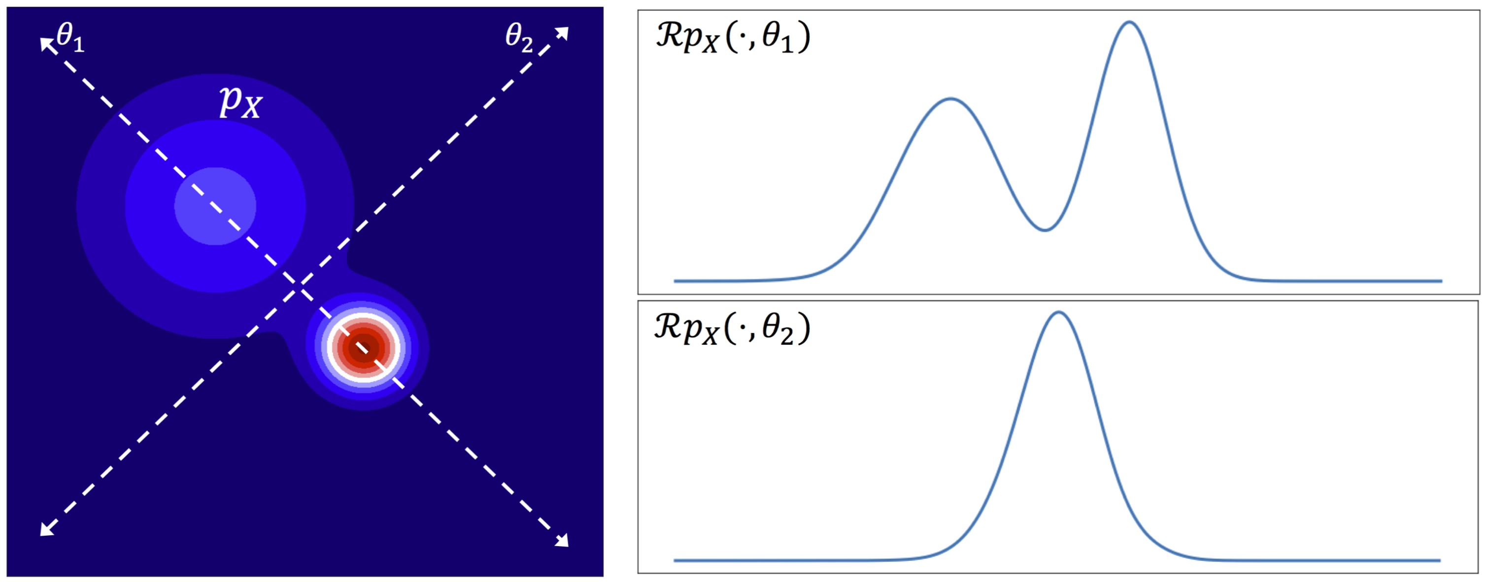
Source: Sliced-Wasserstein Auto-Encoders [3]
I found the following to be a very intuitive interpretation of wasserstein distance in 1D. I would recommend looking at Algorithm 1 box in 2 for a quick overview of how to compute the wasserstein distance.
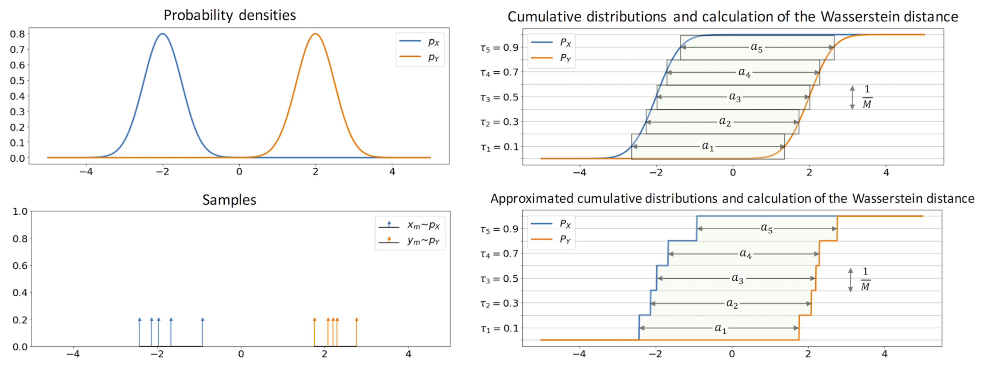
Source: Sliced-Wasserstein Auto-Encoders [3]
Visualizing samples from trained models
In the figure below, I have visualized samples draw from the trained models. Specifically, we are looking at contour plots of densities estimated from model samples. The density of contour lines tells us how steep the modes are, which in case of Target Distribution depends on the choice of mixing coefficients of the GMM.
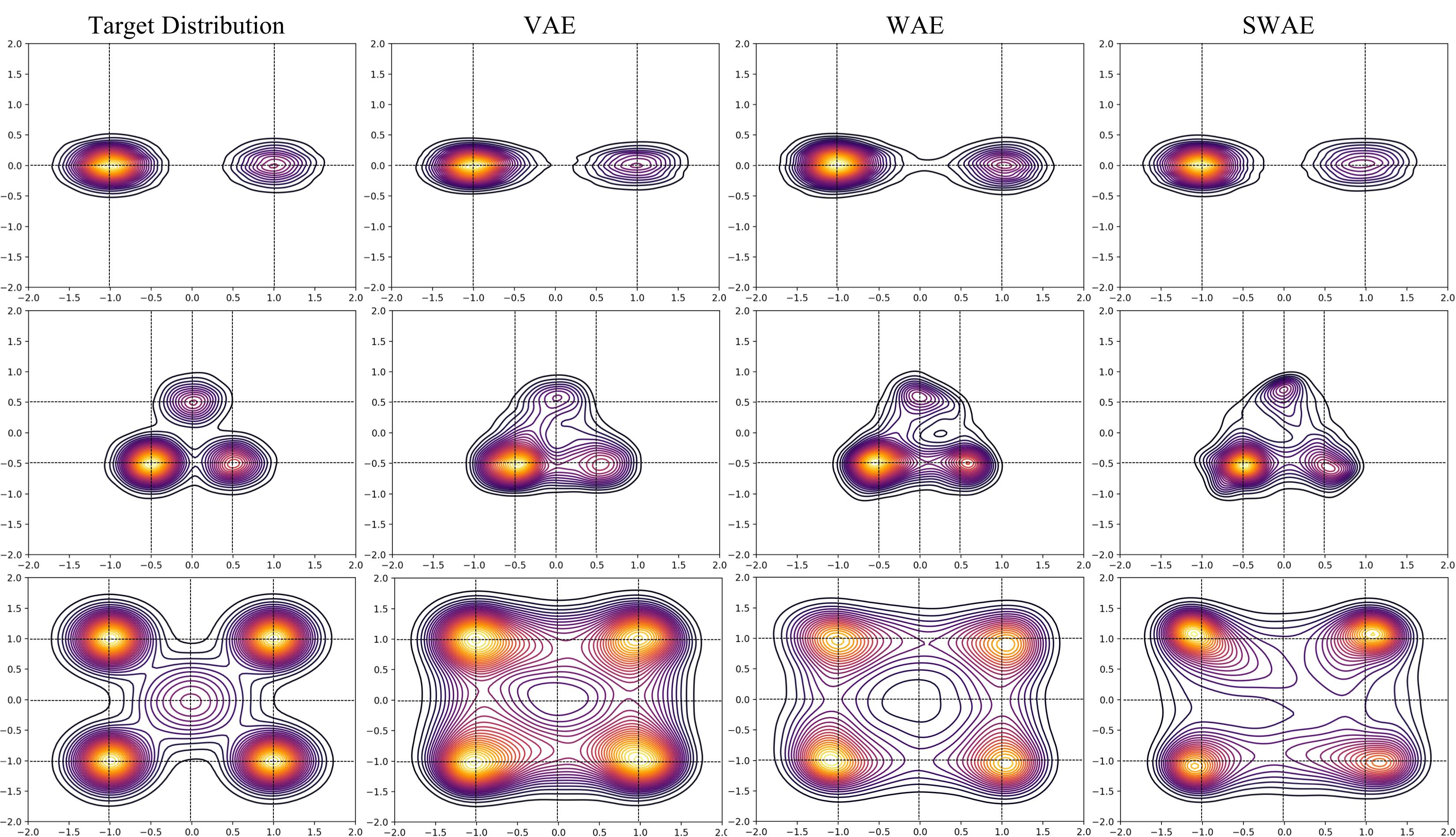
From the plots above, we can make a few observations about the ability of VAE, WAE, and SWAE to learn modes. Modes are the home of the most representative samples from any distribution. Hence it is crucial to check if models learn the location of the modes as well as assign correct densities to those modes.
-
Mode Location: VAE has the most precise mode locations followed by WAE and then SWAE. For instance, see the mode locations
(0.5,-0.5),(0.0,0.5)for the 3 component GMM, and(1,1),(1,-1)for the 5 component GMM. For the 5 component GMM, VAE and WAE missed the low density mode at(0,0). Don’t be fooled by those concentric circles around(0,0)in case of VAE and WAE! Notice how the contour lines get darker as they approach(0,0)indicating a decrease in density as opposed to the increase shown by the target distribution. SWAE doesn’t localize this mode well either but at least the density does not decrease as you approach the mode from most directions. -
Mode density assignment: To gauge density assignment, we need to observe the color (yellow/lighter colors mean higher density), and also the density of contour lines which indicate how steep the peaks are. Note that VAE tends to assign significant density to the space between modes (e.g. around
(0,1)in 5 component GMM) and doesn’t assign significant density to lower density modes like(0.0,0.5),(0.5,-0.5)in 3 component GMM, and(0,0)in 5 component GMM. WAE is slightly unpredictable in density assignment. For instance, WAE assigns too much density to(0.5,-0.5)in the 3 component GMM, and too little to all the high density modes in the 5 component GMM. SWAE’s densities are slightly better calibrated but it has difficulty preserving symmetries both local (around the modes), and global.
Quantitative evaluation using Anderson-Darling statistic
While informative, there is only so much you that you can tell by staring at density plots. In this section, we will present a quantitative evaluation to directly measure how similar the distribution of samples from our models are to samples from the target distributions.
Anderson-Darling statistic is used to test if two set of samples come from the same distribution or if a set of samples is drawn from a given distribution. The AD statistic between two empirical CDFs $F$ (the original distribution of data) and $F’$ (the distribution of samples from learned models) is computed as follows
\[n\int_{-\infty}^{\infty}\frac{(F'(x)-F(x))^2}{F(x)(1-F(x))}dx\]where n is the number of samples used to estimate the empirical CDFs. Basically, the statistic is a weighted sum of squared differences between the two CDFs with higher weights to the tails of the original data CDF. The smaller the value of the statistic, the more confident we can be of the two sets of samples coming from the same underlying distribution.
But our data lives in 2D instead of 1D, so how do we use AD statistic? We slice! We choose a set of random directions and project both sets of samples onto these directions and compute AD statistic in the induced 1D spaces. The 1D statistics are then averaged to get a measure of dissimilarity between the 2D distributions. Note that when comparing different algorithms, we need to be careful to use the same set of random directions for projection.
The following figure compares the AD statistic for the 3 models on the 3 distributions shown above. Smaller the statistic the better. The dotted lines show the lowest AD achieved by each model during training on the test set.
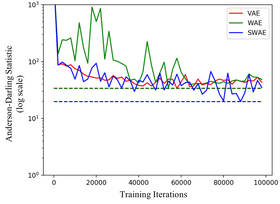
The key observations are as follows:
-
Best achieved performance (the dotted lines): SWAE outperforms VAE in all 3 cases. WAE outperforms VAE in 2 of the 3 cases and performs similarly in case of 5 components.
-
Stability of training: While SWAE and WAE perform similarly in most cases. However, in case of 3 component GMM, we see a sharp rise in AD statistic for WAE around 60000 iterations and the value plateaus to a much larger value than what was already achieved in the first 60000 iterations of training! SWAEs on the other hand are relatively more stable to train.
Encoding Space
AEs and their variants are also commonly used for representation learning. VAEs, WAEs, and SWAEs, all impose constraints on this encoding or representation space. Specifically, they try to match the distribution of samples in the encoding space to that of the prior, which in our case is Standard Normal. The following plots compare the encodings from different models.
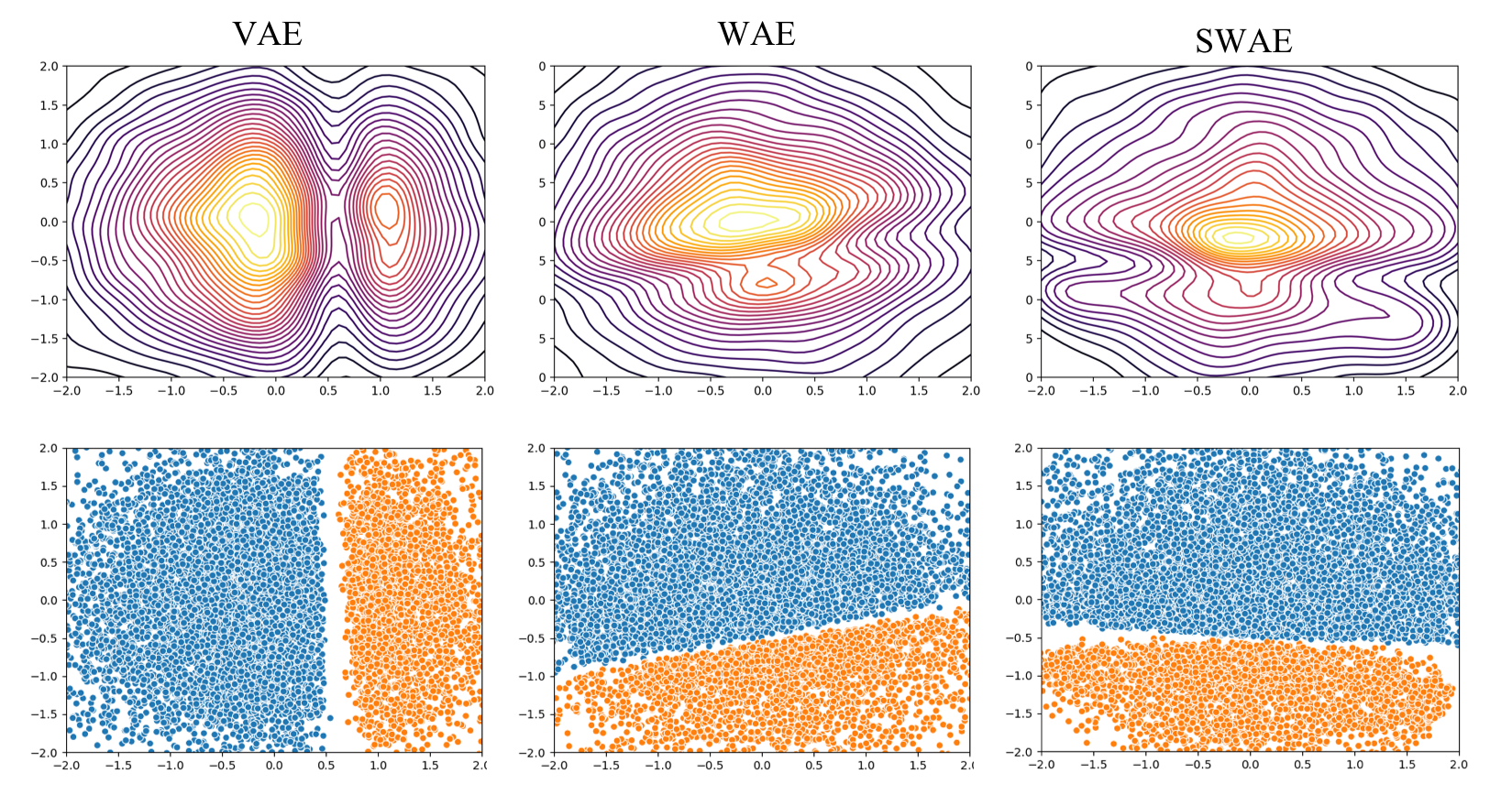
Interestingly, in all cases the components of the GMM remain well separated in the embedding space. In the 2 component case, while VAEs lead to 2 distinct modes in the encoding space, in WAE and SWAE the two modes are merged together in order to match the distribution to the Standard Normal prior. The difference is less visible in 3 and 5 component case.
The Human Factor
Any clever or sophisticated machine learning algorithm is ultimately implemented by a “human” (at least for now). So, it matters what the experience of the person implementing the algorithm is. Does the algorithm simply “work” with a “textbook” implementation at least for toy problems/data like the ones above? Or does the algorithm require “tuning” hyper-parameters? And if so, how sensitive is the algorithm to hyper-parameters - does one need to be roughly in the ballpark to get decent performance or does one need to get them just right? Is there even a signal to guide you to the right hyper-parameters?
In my experience of training these models and assuming a correct implementation, SWAEs start showing meaningful results with typical hyper-parameters! In fact, the only hyper-parameters SWAEs add to AEs is the number of slices and regularization weight. The losses are easy to interpret and help guide the hyper-parameter search. The experience with VAEs was pretty similar except that I had to adjust the weight corresponding to the KL term (the original VAEs did not have this weight but it was introduced later in $\beta$-VAEs5).
WAEs on the other hand were significantly more difficult to find hyper-parameters for. It took me a couple hours and playing with different depths of the discriminator to start seeing results that looked even remotely meaningful. The version that generated results above has a 7 layers deep discriminator which is ridiculous in comparison to my encoder and decoder which are 3 layers deep each. The discriminator is also twice as wide as the encoder and decoder. So SWAEs start appearing quite lucrative when you consider the possibility of loosing the bulky appendage that is the discriminator!
Conclusion
In this post, we discussed the problem with VAEs and looked at WAEs and SWAEs as viable recent alternatives. To compare them we visualized the distributions and encoding spaces learned by these models on samples drawn from three different GMMs. To quantify the similarity of learned distributions to the original distributions, we looked at sliced Anderson-Darling statistic.
Overall, given the conceptual and training simplicity of SWAEs, I personally found them to be a lucrative alternative to VAEs and WAEs. Completely deterministic encoder and decoders, and not requiring a discriminator during learning are two factors going in favor of SWAEs over VAEs and WAEs. SWAEs do have some problems with preserving symmetries, which the VAEs and WAEs are surprisingly good at (especially local symmetry). Hopefully, future research would fix this (one way would be by carefully choosing slicing directions instead of random).
Hope you found the discussion, visualizations and analysis informative! Please feel free to send any feedback, corrections, and comments to my email which you can find here http://tanmaygupta.info/contact/.
References
-
Kingma, Diederik P. and Max Welling. “Auto-Encoding Variational Bayes.” CoRR abs/1312.6114 (2014) ↩
-
Tolstikhin, Ilya O., Olivier Bousquet, Sylvain Gelly and Bernhard Schölkopf. “Wasserstein Auto-Encoders.” CoRR abs/1711.01558 (2018) ↩ ↩2
-
Kolouri, Soheil, Charles E. Martin and Gustavo Kunde Rohde. “Sliced-Wasserstein Autoencoder: An Embarrassingly Simple Generative Model.” CoRR abs/1804.01947 (2018) ↩
-
https://www.deeplearningbook.org/contents/autoencoders.html ↩
-
Higgins, Irina, Loïc Matthey, Arka Pal, Christopher Burgess, Xavier Glorot, Matthew Botvinick, Shakir Mohamed and Alexander Lerchner. “beta-VAE: Learning Basic Visual Concepts with a Constrained Variational Framework.” ICLR (2017). ↩